Parametric and Generative Forecasts of EPEX Day-Ahead Energy Market Curves

Julian Gutierrez; Redouane Silvente

Parametric and Generative Forecasts of EPEX Day-Ahead Energy Market Curves

T0 review · 4 major / 5 minor · reviewed 2026-08-15 · deepseek-v4-flash

Challenge this review Re-run · record.json Download PDF Read on arXiv ↗ Review JSON

Pith's one-line read Order-level diffusion forecasts double a storage operator's expected revenue in the day-ahead market.

desk verdict The bid-level DDPM curve generator is a genuine contribution, but the storage-revenue headline rests on an unvalidated smoothness assumption and an in-sample self-consistency loop. read the letter →

arxiv 2601.20226 v3 pith:C6IKUCHF submitted 2026-01-28 cs.LG cs.SYeess.SY

Julian Gutierrez , Redouane Silvente This is my paper · ORCID

classification cs.LGcs.SYeess.SY

keywords Day-aheadelectricitymarketAggregatedsupplyanddemandcurvesChebyshevapproximationConditionaldiffusionmodelMarkedpointprocessStorageoptimizationPriceimpactDenoisingprobabilisticmodels

verification ladder T0 review T1 audit T2 compute T3 formal

The pith

A machine-rendered reading of the paper's core claim, the machinery that carries it, and where it could break.

The reading

The paper's central claim is that the right object to forecast in the EPEX day-ahead market is not the clearing price but the full supply and demand curves, and that these curves are best captured at the level of the individual buy and sell orders from which they are built. It proposes two complementary tools: a fast parametric model that reduces each curve to eight interpretable parameters (two plateaus and a degree-3 Chebyshev polynomial for the elastic part), and a generative model that treats the order flow as a marked Cox process and samples it with a two-stage conditional diffusion model. The generative model produces plausible curve distributions that, when embedded in a price-maker storage optimization, give about twice the average revenue of the parametric baseline (roughly 61,000 versus 30,000 EUR), with lighter tails near zero and a smaller gap to an oracle benchmark. The contribution is therefore not a new price forecast but curve-forecast machinery that makes storage profitability, price impact, and spread compression quantitatively testable.

What carries the argument

The central object is the marked Cox process encoding of a curve: all distinct prices appearing in the 24 hourly curves are pooled into an ordered grid $(P_m)$, and each price carries a 24-dimensional mark $\Delta S_m$ of volume increments, with zeros where an hour has no offer. A conditional denoising diffusion probabilistic model (DDPM, a neural network trained to reverse gradual noise corruption) learns this process in two stages: first the intensity $\lambda$ given exogenous features, then the marks $\Delta S$ given prices and features. The storage side rests on a second object, the price-impact transfer formula $q_{\mathrm{int}}(P_1,P_2) = (P_1-P_2)/(1/\Gamma'_2(P_2)+1/\Gamma'_1(P_1))$, where $\Gamma_i = D_i - S_i$ is the net demand gap at each hour; it converts predicted curves into the optimal block-order quantity and is what makes the revenue comparison possible.

What would settle it

Take a historical day where the demand-supply gap has a flat segment or jump at prices near the hours' clearing levels, compute the closed-form optimal transfer, and compare it with a brute-force grid search over feasible transfer quantities using the same curves and error samples; if the closed-form quantity has lower expected revenue than the grid optimum, the smooth-invertibility assumption is violated on real data and the reported revenue advantage is not supported.

Watch

Extended reading notes

Core claim

On the paper's own terms, the discovery is that aggregated day-ahead supply and demand curves can be generated order by order: prices arrive as a Cox process whose intensity depends on weather and fuel variables, and each price carries a 24-dimensional volume mark giving the traded volume in every delivery hour. A conditional DDPM in stage one generates the intensity and price arrivals; a second conditional DDPM generates the volume marks; summing the marks reconstructs the hourly curves. The paper shows the generated curves reproduce the inelastic-elastic-plateau structure with average normalized MSE below 1.3% for supply and 5% for demand, and that this probabilistic representation supports a price-maker storage policy. Under the assumption that the demand-minus-supply gaps are smooth, strictly decreasing functions of price, the optimal transfer is given in closed form, and the resulting strategy avoids negative revenues, compresses the spread, and yields higher realized profits than the fast baseline. To the authors' knowledge, this is the first bid-level generative model of day-ahead market curves.

Load-bearing premise

The profit-optimal transfer formula assumes the gap between demand and supply falls smoothly and strictly as price rises, so that the gap function can be inverted and differentiated; real curves with flat plateaus and block-order jumps can violate this, which would break the closed-form policy and the revenue comparison built on it.

Editorial extensions

If this is right

The fast parametric model can be run daily before the noon deadline: five years of training take about a minute on commodity hardware, and a one-hour forecast takes under half a second, with median normalized MAE near 7-11%.
The generative model turns storage revenue from a point estimate into a distribution: across 10,000 forecast-error samples the spread of outcomes is visible, and the model's revenue distribution has lighter tails near zero than the fast baseline.
A price-maker who accounts for its own market impact earns about 27% more than the naive full-capacity arbitrage in the fast-model setting, and the generative model roughly doubles that average revenue to about 61,000 EUR for the case study.
Large storage deployment compresses the price spread: peak-hour prices fall, off-peak prices rise, and beyond roughly 1,500 MW of transfer capacity the marginal benefit shrinks so much that payback times exceed ten years.
Because the generative model conditions only on weather and fuel prices, it can be used for multi-day scenario analysis, not just next-day bidding, by aggregating samples across days.

Reading between the lines

Editorial extensions of the paper, not claims the author makes directly.

A testable extension is to feed the fast model's point forecast with noise drawn from the generative calibration and compare revenues; this would separate how much of the doubling comes from curve realism versus the shape of the error distribution.
The paper leaves linked block orders and minimum-income conditions out of scope; applying the same marked-process decomposition to intraday auctions, where these constraints matter more, would show whether order-level generation transfers to richer market mechanisms.
The reported revenue comparison assumes independence between forecast errors at the two hours; coupling the error variables with a copula would quantify how much of the profit advantage survives correlation.
An oracle benchmark that replaces predicted curves with realized curves would isolate the value of forecast accuracy from the value of the price-impact policy, a decomposition the paper does not report.

Share X Bluesky LinkedIn Reddit HN

Signed reviews

No signed human review yet.

Editorial analysis

A structured set of objections, weighed in public.

Desk editor's note, referee report, and a circularity audit.

Desk Editor's Note

read the letter

Here's my take. The genuine contribution is the order-level generative model: treating each day's supply and demand curves as realizations of a marked Cox process, learning price arrivals and volume marks with two-stage conditional DDPMs, and then aggregating synthetic orders into full curves. That is new in the day-ahead curve literature, which mostly works on fixed grids or low-dimensional parametric forms. The fast parametric baseline is also well executed: eight interpretable parameters, Chebyshev polynomials, monotonicity enforced, fast training, and a sensible comparison against naive persistence. The storage optimization math in Section 4.1 is coherent as a theoretical exercise.

The soft spots are real and, in my reading, load-bearing for the paper's headline claims. Assumption 4.2 requires each net demand curve Gamma_i to be C1 and strictly decreasing. But the curves used in the application are step functions or piecewise-flat reconstructions: the generative model aggregates discrete orders, and the parametric model enforces monotonicity via cumulative minima, producing flat plateaus and kinks. On any flat segment, Gamma' is zero, the inverse is set-valued, and the closed-form q_int in Corollary 4.1 divides by 1/Gamma', which is undefined. The paper never checks Assumption 4.2 on the curves actually fed into the optimizer. Since Figure 40 shows interior solutions occurring in a substantial share of scenarios, this is not an edge case.

Separately, the "higher realized profits" claim in the abstract is not realized in the empirical sense. The comparison uses one date, 2020-10-05, with errors sampled from distributions fitted to the model's own residuals and with the model's mean curves placed in the equilibrium equations. That is a self-consistency loop, not an out-of-sample test. The oracle benchmark mentioned in the abstract is never defined in the full text. There is also a date inconsistency: the abstract says French EPEX data 2021-2024, but the generative model is trained on 2017-2020 and the case study is 2020.

On balance, the paper deserves serious refereeing. The modeling idea is strong enough that a careful referee should see it through, but the empirical validation needs major revision: check Assumption 4.2 on real curves, run a proper out-of-sample revenue evaluation, define the oracle, and align the stated data periods. I would not rely on the revenue numbers as they stand, but I would cite the bid-level generative representation if I worked in this area.

Referee Report

4 major / 5 minor

Summary. The paper proposes two curve-forecasting frameworks for the EPEX SPOT day-ahead market: a fast parametric model that represents each hourly demand/supply curve by a small set of parameters (plateaus, Chebyshev polynomial coefficients, and elastic-region boundaries) predicted by XGBoost, and a generative model that treats curves as aggregations of individual orders modeled as a marked Cox process with prices and volumes generated by conditional denoising diffusion probabilistic models. The forecasts are used in a price-maker storage optimization between an off-peak and a peak hour, where a closed-form optimal transfer quantity is derived from supply/demand net-curve assumptions. The authors evaluate reconstruction accuracy and compare storage revenues from the parametric and generative frameworks, reporting a two-fold higher average revenue for the generative model and a price-compression effect of storage, with payback-time analysis.

Significance. If the empirical claims were supported, the paper would be a useful contribution to curve-based electricity price forecasting and storage optimization, particularly the bid-level generative approach via marked point processes and diffusion models. The parametric representation is interpretable and computationally light, and the generative framework is a novel attempt at probabilistic, order-level day-ahead curve simulation. The storage application with price impact is thematically relevant. However, the paper's central empirical claims are currently not validated: the revenue comparison rests on a single date under the model's own error distribution, the oracle benchmark is undefined, and the theoretical derivation relies on a smoothness assumption that the applied curves do not satisfy. The generative model also does not consistently outperform the fast baseline in the distributional evaluations. The paper ships no code or machine-checked proofs, so the reported numbers are the only evidence.

major comments (4)

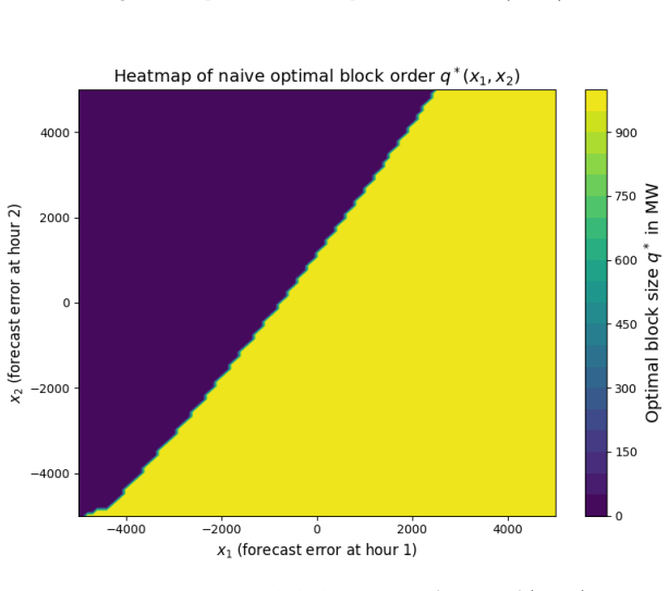
[Section 4 / Assumption 4.2 and Corollary 4.1] Assumption 4.2 requires Gamma1 and Gamma2 to be C1 and decreasing, which guarantees invertibility and uniqueness of equilibrium prices. The curves used in Section 4.2.2 do not satisfy this assumption: the fast parametric model enforces monotone non-increase via np.minimum.accumulate, producing flat plateaus and kinks, and the generative model of Section 3 aggregates order-level step functions, which are discontinuous with derivative zero almost everywhere. On any flat segment Gamma'_i = 0, the expression in Corollary 4.1 divides by 1/Gamma'_i, and Gamma_i^{-1} is set-valued. The manuscript never checks the assumption on the curves actually used, and Figure 40 shows interior solutions occur in a substantial share of scenarios, so the violation is material. As written, the closed-form optimal transfer q_int and the reported revenue comparison are not validly derived.
[Abstract and Section 4.2.2] The abstract claims 'higher realized profits and smaller gaps to an oracle benchmark', but no oracle is defined anywhere in the manuscript, and the profits are computed as expected revenues using the model's own calibrated forecast-error distribution X (fitted to the model's residuals over 2020) rather than as realized profits on actual market outcomes. The evaluation is a self-consistency loop: mean curves from the generative model are fed into the equilibrium, errors are sampled from a distribution fitted to that same model's residuals, and expected profits are reported. This does not constitute validation on realized market outcomes and does not support the phrase 'realized profits'.
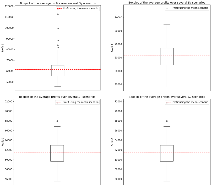
[Section 4.2.2] The headline comparison of the fast and generative models (approximately 30,000 versus 61,000 EUR average revenue) is based on a single date, 2020-10-05. With one evaluation date, the two-fold improvement is not statistically grounded and could reflect a single favorable scenario rather than a systematic advantage. The authors should evaluate over multiple out-of-sample dates, report confidence intervals or standard errors, and compare against actual realized payoffs rather than model-generated expectations.
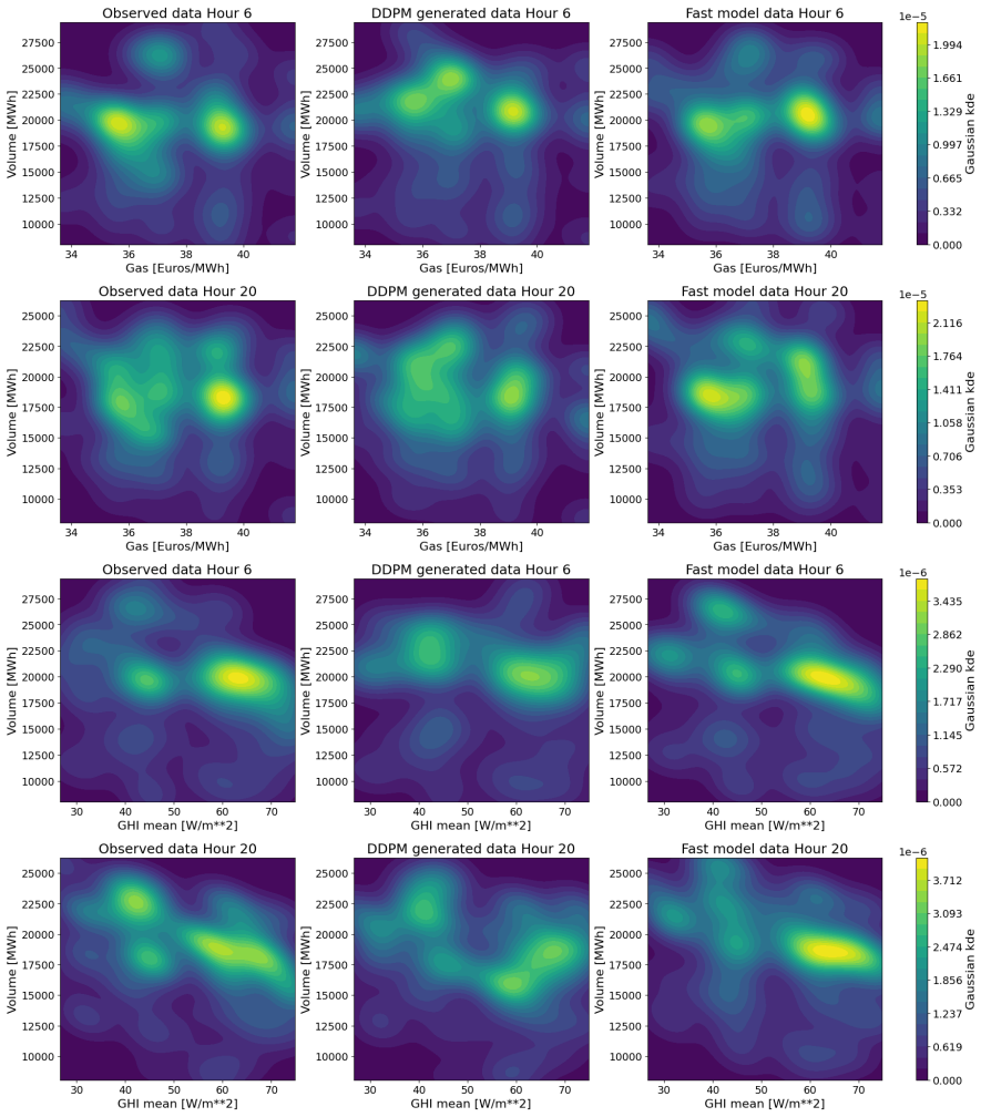
[Section 3.2] The generative model's reconstructive and distributional performance is evaluated on a very limited temporal basis: normalized MSE on a single date (2020-10-05) and Wasserstein distances on one month (January 2020) for two hours. The Wasserstein results in Figures 27-29 show that the fast model often outperforms or matches the DDPM, and the DDPM only beats the fast model for hour 20 in the elastic region. This does not support a general claim of superior realism for the generative model and should be tempered or expanded with multi-month, multi-hour evaluation.

minor comments (5)

[Section 2.1] Algorithm 1 uses the 90th percentile of finite-difference slopes to detect the elastic segment; this is a free parameter whose sensitivity is not discussed. A sentence on its stability would be useful.
[Section 3.2] The text says the average normalized MSE 'stays below 1.3% (5% for the demand)', but it is not immediately clear which percentage applies to which curve type; please label the supply and demand results explicitly in the text and figure.
[Section 4.2.2] The paper calibrates X using the mean of 10 generated curves but reports revenue computations using means over 100 generated samples; the reason for this discrepancy and its effect on the calibrated error distribution should be explained.
[Title and abstract] The running title on the arXiv header is 'Parametric and Generative Forecasts of EPEX Day-Ahead Energy Market Curves', while the full-text title is 'Parametric and Generative Forecasts of Day-Ahead Market Curves for Storage Optimization'; these should be harmonized. The abstract also introduces an 'oracle benchmark' that is never defined in the body; either define it or remove the phrase.
[Section 3.1.2] The Gaussian perturbation of zero volume marks (N(-50,5) for supply and N(50,5) for demand) introduces a sign asymmetry whose effect on generated curves is not analyzed; a sentence on why the mean is offset below or above zero would improve interpretability.

Circularity Check

1 steps flagged · score 6.0 of 10

The headline storage-profit claim is a self-consistency loop: the error distribution and the equilibrium curves both come from the same model, so the two-fold revenue advantage is constructed from the model's own fitted inputs rather than from realized market outcomes.

fitted input called prediction [Section 4.2, Calibration of X, Eq. (10); Section 4.2.2, Comparison of the revenue distribution]
"Xd,h =D predd,h (Pobsd,h )−S predd,h (Pobsd,h ).(10) This definition assesses the prediction models exactly where accuracy matters the most: at the market-clearing price. [...] We calibrate X against the generative model, taking Spredd,h and D predd,h as the mean of 10 supply and demand curves generated in Section 3. [...] The first observation is that the average revenue obtained is 2 times higher (approx. 30 000 to 61 000 EUR)."

Equation (10) defines the forecast error X as the gap of the model's own predicted curves at the observed price. In Section 4.2.2 those predicted curves are the generative model's own mean curves, and the same curves are inserted into the market-clearing equation (6) to solve equilibrium prices and revenues. For q=0, (6) becomes Gamma(P)=X=Gamma(P_obs), so by construction the model reproduces the observed price; the 10,000 revenue draws are then generated from a distribution fitted to these same residuals. The reported two-fold revenue advantage (30,000 vs 61,000 EUR) therefore measures each model's own fitted residuals against its own forecast curves, not realized market outcomes. Calling this 'realized profits' in the abstract is a fitted input renamed as a prediction.

full rationale

The main forecasting content is not circular: the generative model is scored against historical curves (normalized MSE, Wasserstein distances), and the authors explicitly state it does not consistently outperform the fast baseline; the parametric model is evaluated out-of-sample on 2024. The self-citation to Dumitrescu et al. (2024), co-authored by Silvente, is used only as supporting literature for the spread-compression and cannibalization effects and is not load-bearing. However, the headline profit claim is circular in a narrower sense. X is calibrated by Eq. (10) on each model's own predicted curves at observed prices, and the same predicted curves are then plugged into Eq. (6) to solve the storage equilibrium and simulate 10,000 revenue draws. Because for q=0 the equilibrium equation reduces to Gamma(P)=X=Gamma(P_obs), the model is made to reproduce observed prices by construction; the revenue simulations therefore measure each model's fitted residuals against its own forecast curves rather than realized market outcomes. The abstract's 'realized profits' and the two-fold revenue advantage are thus a self-consistency loop, not an external validation. Separately, Assumption 4.2 (C1, strictly decreasing Gamma) is not checked for the step-function curves used, and the abstract's oracle benchmark is never defined; these are validity or correctness gaps rather than circularity, but they reinforce that the revenue comparison is not an independent empirical result. Overall, partial circularity centered on the storage profit claim.

Assumptions & free parameters 8 free parameters · 6 assumptions · 0 invented entities

The paper introduces no new physical or ontological entities. The surrogate intensity lambda is an internal statistical construct, and the latent variables Z and Z' are standard generative-model latents, not independently testable entities. The free parameters above are the hand-set thresholds, grid choices, noise scales, and fitted error distributions that the central claims depend on.

free parameters (8)

Algorithm 1 slope quantile threshold (pct=90) = 0.90
Defines the elastic-region boundaries p_start and p_end; all downstream curve predictions depend on this hand-set quantile.
Chebyshev degree for elastic segment = 3
Degree 3 chosen after comparing degree 5/7 and sigmoid alternatives; retained as an accuracy and simplicity compromise.
Price-arrival intensity grid allocation = 30 points: 5 on (0,0.1), 20 on [0.1,0.3], 5 on (0.3,1]
Grid allocation for the surrogate lambda chosen after extensive testing; affects thinning and generated price arrivals.
Volume-mark DDPM split thresholds = 200 MWh supply, 450 MWh demand
Chosen by numerical trials as the best empirical performance; splits marks into low-volume and high-volume models.
Zero-replacement Gaussian noise parameters = Supply N(-50,5) and N(-250,25); demand N(50,5) and N(250,25)
Replaces the Dirac mass at zero with small-variance Gaussians; selected after repeated trials to balance separation and symmetry.
DDPM sampling parameter alpha = 1/3
Used in Algorithm 2 reverse sampling; value fixed in Section 3.1.1 without a stated optimization.
Calibrated forecast-error distributions for storage optimization = Fast: N(555, 2300) and Laplace(1367, 1896); generative: SkewNorm(4.86, 1149, 6680) and SkewNorm(3.65, 2265, 5466)
BIC-selected families and parameters fitted to each model's residuals; they directly determine the revenue distributions reported in Section 4.2.
Storage case-study parameters = qM=1000 MW, cdeg=30 EUR/MWh
Fix the illustrative storage unit and degradation cost; payback and cannibalization results scale with these choices.

assumptions (6)

domain assumption Aggregate day-ahead curves have a plateau-elastic-plateau shape with two flat segments and a monotone elastic middle.
Basis of the eight-parameter reduction in Section 2.1; not universally guaranteed when block orders and price caps distort curves.
domain assumption Order arrivals form a marked Cox process with stochastic intensity lambda; volume marks are conditionally independent given price and features.
Section 3.1 model for supply and demand orders; linked block and minimum-income orders are explicitly excluded.
domain assumption Forecast errors X_{d,h} admit a density and are independent across hours (Assumption 4.1).
Used to compute expected revenue products and pointwise optimal q*(x1,x2); the paper acknowledges a correlation gap if relaxed.
domain assumption Net demand-supply differences Gamma1 and Gamma2 are C1 and strictly decreasing (Assumption 4.2).
Guarantees invertibility and uniqueness of equilibrium; flat plateaus or block discontinuities violate it and break Corollary 4.1.
ad hoc to paper DDPMs approximate smooth continuous densities; the Dirac mass at zero must be smoothed before training.
Section 3.1.2 replaces zero marks with Gaussian noise; the noise scale is an added modeling assumption not derived from data.
standard math Time-rescaling theorem and standard optimal transport or Chebyshev results are valid for the constructed surrogates.
Used for lambda fit diagnostics and Wasserstein comparisons; standard results, but their applicability to the surrogate data is assumed.

how reviews work

0 comments

Cite this review

Pith. "Pith review of Parametric and Generative Forecasts of EPEX Day-Ahead Energy Market Curves." pith.science (2026). https://pith.science/paper/C6IKUCHF

@misc{pith2026260120226,
  author       = {Pith},
  title        = {Pith review of: Parametric and Generative Forecasts of EPEX Day-Ahead Energy Market Curves},
  year         = {2026},
  howpublished = {\url{https://pith.science/paper/C6IKUCHF}},
  note         = {Machine review of arXiv:2601.20226}
}

read the original abstract

We propose two methodologies for modelling aggregated supply and demand curves in the EPEX SPOT Day-Ahead market, emphasizing generative models as a way to recover distributional variability. The first is a low-dimensional parametric representation that yields deterministic point forecasts; the second is a high-dimensional order-level representation that samples from a conditional distribution of plausible curves. Both model the full curve structure, enabling the analysis of price sensitivity, volume sensitivity, and price impact. The parametric representation uses plateau levels, elastic-region boundaries, and polynomial coefficients, forecast with eXtreme Gradient Boosting. The main contribution is the generative representation, which uses price arrivals and volume-increment marks and is implemented with conditional Denoising Diffusion Probabilistic Models. Using French EPEX data from 2021 to 2024, we evaluate both approaches through curve reconstruction and a price-maker storage optimization problem. The parametric implementation provides a deterministic reference, while the diffusion-based implementation produces distributions of plausible curves and achieves higher realized profits and smaller gaps to an oracle benchmark in the storage application.