REVIEW 2 major objections 7 minor 3 cited by
Two staggered 'projector splitting' schemes for low-rank approximations of SDEs converge with constants independent of the smallest singular value, removing the restrictive time-step condition of DLR Euler–Maruyama.
Reviewed by Pith at T0; open to challenge. T0 means a machine referee read the full paper against a public rubric. the ladder, T0–T4 →
Three time-stepping schemes for dynamically-orthogonal low-rank SDE surrogates are introduced; two projector-splitting variants converge with bounds independent of the smallest singular value.
T0 review reviewed 2026-08-03 challenge →
load-bearing objection First rigorous time-discretization analysis for DLRA-SDEs, with useful staggered schemes, but one of the two central convergence theorems has a bound that does not actually imply convergence. the 2 major comments →
Numerical Methods for Dynamical Low-Rank Approximations of Stochastic Differential Equations -- Part I: Time discretization
The pith
A machine-rendered reading of the paper's core claim, the machinery that carries it, and where it could break.
The reading
Core claim
The central result is that the DLR Projector Splitting for Euler–Maruyama satisfies √E[sup_{0≤s≤t}|X_ns - X_true(s)|^2] ≤ C(√E|X_0 - X_true_0|^2 + Δt^{min{1/2,α}} + ε + ε/√Δt), with C independent of the smallest singular value of the covariance matrices of the stochastic modes. The DLR Projector Splitting for SDEs enjoys a similar bound with the ε/√Δt term removed, because only the drift is projected onto the tangent space in the deterministic-mode update, making the scheme adapted to the natural filtration. The paper also shows that, under non-degenerate noise, the stochastic-mode Gramian stays positive definite with an explicit lower bound for all three schemes, and that the two staggered
What carries the argument
The Dynamically Orthogonal / dynamical low-rank ansatz X = U^T Y, with orthonormal deterministic modes U and stochastic modes Y, leads to the Gramian C_Y = E[Y Y^T] whose inverse appears in the equation for the deterministic modes. The staggered schemes replace the simultaneous forward update by: first evolve Y with Euler–Maruyama using the current U, then compute the new deterministic modes using the freshly computed stochastic modes and a tangent-space projector P_{U^T Y~}, followed by QR orthonormalization. This projector-splitting structure is what removes the dependence on the smallest singular value of the Gramian.
Load-bearing premise
The proofs assume that every expectation inside Algorithms 1–3 is computed exactly at each time step; the numerical experiments instead use Monte Carlo sample averages, and the analysis does not control that replacement.
What would settle it
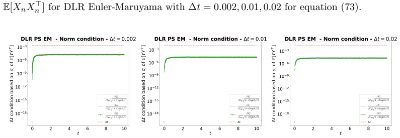
Repeat the Section 7 experiments for the staggered schemes on problem (70) with σB=10^-19 so the stochastic-mode Gramian hovers near machine zero; if the strong error, or the Δt needed to reach a fixed tolerance, grows like 1/σ_min as the smallest singular value decreases, the claimed independence from the singular value is wrong.
If this is right
- DLR Euler–Maruyama is usable when Δt meets the singular-value-dependent condition; under non-degenerate noise the Gramian remains full rank with a lower bound matching the continuous case.
- The two staggered schemes converge strongly to the true SDE solution with order min{1/2,α} plus a low-rank projection error ε; for DLR Projector Splitting for SDEs the bound does not include the ε/√Δt term.
- Both staggered schemes are mean-square stable for linear SDEs under the same sufficient condition as standard Euler–Maruyama, independent of the smallest singular value of the stochastic Gramian.
- No time-step restriction is needed for the L2 norm bound of the staggered schemes, so near-rank-deficient stochastic modes do not halt the computation.
- Algorithm 3's update is adapted to the filtration, making it the natural target for the Monte Carlo discretization treated in Part II.
Where Pith is reading between the lines
- If Part II justifies Monte Carlo replacement of expectations with rigorous error control, the projector-splitting schemes become immediately usable in large-scale uncertainty quantification; until then the proven rates apply only to the idealized exact-expectation algorithms.
- The ε term in the error bound is a computable measure of how far the drift and diffusion are from the tangent space of rank-k processes, so it could be used adaptively to grow or shrink the rank during a simulation.
- Because the deterministic-mode update in linear-drift cases decouples from the Gramian, the staggered schemes may parallelize across stochastic samples or combine with rank-adaptive integrators without triggering step-size crashes.
- The experiments with nearly singular Gramians suggest the staggered schemes may tolerate stochastic modes whose Gramian becomes numerically singular, a regime where classical DLRA integrators for deterministic problems typically require regularization.
Editorial analysis
A structured set of objections, weighed in public.
Referee Report
Summary. The paper proposes and analyzes three time-discretization schemes for the Dynamically Orthogonal (DO) formulation of dynamical low-rank approximation (DLRA) for high-dimensional SDEs. Algorithm 1 (DLR Euler–Maruyama) is shown to converge under a time-step restriction tied to the smallest singular value of the Gramian; Algorithms 2 and 3 are staggered projector-splitting variants designed to remove that restriction. The paper proves moment bounds, non-degeneracy of the Gramian under non-degenerate noise, mean-square stability for linear SDEs, and strong convergence estimates comparing the numerical DLR solution both to the continuous DLRA solution and to the exact SDE solution. Numerical experiments with Monte Carlo expectations are provided for low-dimensional SDEs and for discretized SPDEs.
Significance. If the results are correct, this is a useful contribution: it extends the DLRA time-discretization theory from deterministic/random PDEs to general SDEs, gives explicit convergence rates, identifies the singular-value dependence of the standard Euler–Maruyama approach, and proposes staggered schemes with better robustness. The paper is careful to state that all expectations are exact in the theory and to defer Monte Carlo sampling to Part II. The proofs are detailed and are derived from stated assumptions with no fitted parameters. However, the central convergence claim for Algorithm 2 is not established as stated because the error bound in Theorem 5.5 contains an ε/√Δt term that diverges as Δt→0 for fixed modeling error ε>0. This is a load-bearing defect in one of the paper's headline contributions.
major comments (2)
- [Theorem 5.5 / Proposition 5.3] The advertised convergence of Algorithm 2 is not established. In the proof of Proposition 5.3, the diffusion term T2 is bounded by repeatedly applying Cauchy–Schwarz and then using E[|Y~_{n+1}^T C_{Y~_{n+1}}^{-1} Y~_{n+1}|]=k for each of the n_t summands. This yields the displayed bound ε²Δt n_t E[Σ |C_{Y~_{n+1}}^{-1/2}Y~_{n+1}|²] ≤ ε²T²/Δt. Passing to the square root gives the ε/√Δt term in Theorem 5.5. For any fixed positive modeling error ε>0, this term diverges as Δt→0, so the right-hand side has no finite limit and the theorem does not imply convergence in time. This is not a Monte Carlo issue; it fails at the exact-expectation level. The estimate discards the martingale-difference structure of the Brownian increments: a sharper bound exploiting the summation structure is needed to obtain O(ε) rather than O(ε/√Δt). As stated, Theorem 5.5 cannot support the abstract's claim that the
- [Section 6, Theorem 6.3] Theorem 6.3 is stated without proof. This theorem is a central convergence result for Algorithm 3 and is the source of the clean ε dependence that contrasts with Algorithm 2. The section says only that the results are obtained 'via similar proofs,' but no proof or even a detailed sketch is provided. In particular, the reader cannot verify how the ε/√Δt factor is avoided. Please provide the proof or a precise sketch, especially the treatment of the diffusion term that leads to the O(ε) bound.
minor comments (7)
- [Proposition 4.1] The vector v is first taken in R^d ('Let us take a unit vector v ∈ R^d') but the Gramian CY_{n+1} is k×k and later the infimum is over v∈R^k. This should be corrected to avoid confusion.
- [Lemma 4.2 proof] The treatment of T5 is incomplete: after 'For T4 one obtains' there is no displayed bound for T5, and the final line labels the term as T4+T5 without showing the T5 estimate. Please add the missing derivation or state explicitly that it is analogous to T4.
- [Theorem 4.7 proof] In the line after (46), the factor is written 'expmax(A,B)T ·2(C + D)((Δt)^{min{1,2α}})' which is ambiguous. It should be exp(max{A,B}T)·2(C+D)(Δt)^{min{1,2α}} (or similar).
- [Section 5] The text says 'This result is subsequently applied in Proposition 5.1' but the result referred to is Proposition 5.2. The cross-reference should be corrected.
- [Section 7.3] The first occurrence of 'Figures 14, 15, and 16' in Section 7.3 should instead refer to Figures 10–12; the same figure numbers are reused in Section 7.4. Please fix the figure references.
- [Conclusion / Numerical experiments] All theorems assume exact expectations, while Section 7 replaces them with Monte Carlo sample averages. The conclusion acknowledges this and defers the analysis to Part II, but a sentence in Section 7 clarifying that the numerical plots validate the combined time-and-sample discretization (not the time discretization alone) would help prevent over-reading of the empirical convergence rates.
- [Theorem 5.5] The theorem says 'Suppose Assumptions (1)-(2) hold' but the Assumptions are numbered 1–3; please update the reference.
Circularity Check
No significant circularity: the convergence estimates are new derivations; reliance on the authors' prior continuous DLRA theory is normal, non-load-bearing self-citation, though Theorem 5.5's ε/√Δt term and the exact-expectation/Monte-Carlo gap are non-circular limitations.
full rationale
I found no circular step that makes a prediction equivalent to its inputs by construction. The DO equations are taken from the authors' prior work [18] and the projector-splitting perspective from [16,17,27], but all new convergence bounds (Theorems 4.7, 4.10, 5.3, 5.5, 6.3, 6.4) are obtained from the stated Lipschitz, linear-growth, uniform-ellipticity, Hölder-in-time, and rank-k projection-error assumptions via Gronwall/Doob/Itô arguments. The quantity ε in (47) is a best-approximation projection error, not a fitted parameter, so its appearance in the error bounds is not circular. The paper explicitly flags the exact-expectation restriction in the conclusion: 'all the analyses done in this first part always assumes exact expectations for Algorithms 1, 2, and 3', while Section 7 uses Monte Carlo averages; this is an acknowledged gap, not a disguised reuse of inputs. The self-citations to [16,18] supply well-posedness and technical lemmas for the continuous DLRA; they are parameter-free results with stated assumptions and are not the target discretization claims, so they do not create a self-citation chain that forces the present results. One non-circular correctness caveat should be flagged: in Proposition 5.3, the T2 estimate is bounded by replacing a sum of n_t terms with a Cauchy–Schwarz factor n_t, yielding 3ε²T²/Δt, so Theorem 5.5 contains the term ε/√Δt, which diverges as Δt→0 for fixed ε>0. Thus Algorithm 2's advertised convergence is not established by that bound; this is a proof-strength issue, not circularity, and Algorithm 3's Theorem 6.3 (with plain ε) is not affected. Overall, no load-bearing circular step; only minor, non-load-bearing self-citation.
Axiom & Free-Parameter Ledger
axioms (8)
- domain assumption Drift and diffusion are uniformly Lipschitz continuous (Assumption 1, Eq. (3)).
- domain assumption Drift and diffusion satisfy linear growth bound (Assumption 2, Eq. (4)).
- domain assumption Initial condition is square integrable and F0-measurable (Assumption 3).
- domain assumption Initial Gramian CY0 is invertible (Assumption 4).
- domain assumption Non-degenerate diffusion: b b^T ⎷ σB I (Assumption 5).
- domain assumption Hölder continuity in time of drift and diffusion (Eq. (41)).
- domain assumption Bounded rank-k projection error ε (Eq. (47)).
- domain assumption All expectations in Algorithms 1–3 are computed exactly.
Cite this review
Pith. "Pith review of Numerical Methods for Dynamical Low-Rank Approximations of Stochastic Differential Equations -- Part I: Time discretization." pith.science (2026). https://pith.science/paper/E4A4EZOY
@misc{pith2026260121428,
  author       = {Pith},
  title        = {Pith review of: Numerical Methods for Dynamical Low-Rank Approximations of Stochastic Differential Equations -- Part I: Time discretization},
  year         = {2026},
  howpublished = {\url{https://pith.science/paper/E4A4EZOY}},
  note         = {Machine review of arXiv:2601.21428}
}
read the original abstract
In this work (Part I), we study three time-discretization schemes for the Dynamical Low-Rank Approximation (DLRA) of high-dimensional stochastic differential equations (SDEs). Specifically, we consider the Dynamically Orthogonal (DO) method for DLRA proposed and analyzed in arXiv:2308.11581v4, which approximates the true solution by a linear combination of few products between deterministic orthonormal modes and stochastic modes, both time-dependent. The first scheme considered consists in a forward discretization in time of both deterministic and stochastic components, in a Euler-Maruyama style. Its convergence is proven subject to a time-step restriction dependent on the smallest singular value of the Gram matrix associated to the stochastic modes, which, on its turn, is shown to be always positive, provided that the SDE under study is driven by a non-degenerate noise. The second and the third schemes, on the other hand, are staggered ones, alternating updates of the deterministic and the stochastic modes in half steps, and have a projector splitting nature. We show stability of the second scheme and prove convergence with constants independent of the smallest singular value. The third scheme works better in practice, although our theoretical convergence bounds are worse than those for the second one. Computational experiments support our theoretical results. In this work we do not consider the discretization in probability, which will be the topic of Part II.
Figures




Forward citations
Cited by 3 Pith papers
-
Dynamical Low-Rank Filters for Data Assimilation
Dynamical low-rank filters minimize joint mean-covariance error for SDE data assimilation and extend to Kalman-Bucy, ensemble, and particle forms for nonlinear problems.
-
Long-time Behaviour of DLRA for SDEs
Proves existence of invariant measures for strong DO systems approximating SDEs via moment estimates and fixed-point arguments under standard dissipativity assumptions.
-
Dynamical Low-Rank Smoothing
DLRA-JMCO filtering is extended via RTS recursion to a reduced-order smoother, with a Kalman–Bucy form for affine drift, cutting cost and storage while keeping an adaptive low-rank basis.
Reference graph
Works this paper leans on
-
[1]
Modeling with Itˆ o stochastic differential equations
Edward Allen. Modeling with Itˆ o stochastic differential equations. Vol. 22. Springer Science & Business Media, 2007
2007
-
[2]
Stochastic differential equations
Ludwig Arnold. Stochastic differential equations. John Wiley, New York (NY), 1974
1974
-
[3]
Existence of dynamical low-rank approximations to parabolic problems
Markus Bachmayr, Henrik Eisenmann, Emil Kieri, and Andr´ e Uschmajew. “Existence of dynamical low-rank approximations to parabolic problems”. In: Mathematics of Computation 90.330 (2021), pp. 1799–1830
2021
-
[4]
Interpola- tory Dynamical Low-Rank Approximation: Theoretical Foundations and Algorithms
Benjamin Carrel, Daniel Kressner, Hei Yin Lam, and Bart Vandereycken. “Interpola- tory Dynamical Low-Rank Approximation: Theoretical Foundations and Algorithms”. In: arXiv preprint arXiv:2510.19518 (2025)
arXiv 2025
-
[5]
A rank-adaptive robust integra- tor for dynamical low-rank approximation
Gianluca Ceruti, Jonas Kusch, and Christian Lubich. “A rank-adaptive robust integra- tor for dynamical low-rank approximation”. In: BIT Numerical Mathematics (2022), pp. 1–26
2022
-
[6]
An unconventional robust integrator for dy- namical low-rank approximation
Gianluca Ceruti and Christian Lubich. “An unconventional robust integrator for dy- namical low-rank approximation”. In:BIT Numerical Mathematics 62.1 (2022), pp. 23– 44
2022
-
[7]
Stochastic equations in infinite dimensions
Giuseppe Da Prato and Jerzy Zabczyk. Stochastic equations in infinite dimensions . Vol. 152. Cambridge university press, 2014
2014
-
[8]
A low-rank projector-splitting integrator for the Vlasov–Poisson equation
Lukas Einkemmer and Christian Lubich. “A low-rank projector-splitting integrator for the Vlasov–Poisson equation”. In: SIAM Journal on Scientific Computing 40.5 (2018), B1330–B1360
2018
-
[9]
A robust and con- servative dynamical low-rank algorithm
Lukas Einkemmer, Alexander Ostermann, and Carmela Scalone. “A robust and con- servative dynamical low-rank algorithm”. In: Journal of Computational Physics 484 (2023), p. 112060
2023
-
[10]
On the Dirac–Frenkel vari- ational principle on tensor Banach spaces
Antonio Falc´ o, Wolfgang Hackbusch, and Anthony Nouy. “On the Dirac–Frenkel vari- ational principle on tensor Banach spaces”. In: Foundations of computational mathe- matics 19 (2019), pp. 159–204
2019
-
[11]
Low-order stochastic mode reduction for a realistic barotropic model climate
Christian Franzke, Andrew J Majda, and Eric Vanden-Eijnden. “Low-order stochastic mode reduction for a realistic barotropic model climate”. In: Journal of the atmo- spheric sciences 62.6 (2005), pp. 1722–1745
2005
-
[12]
Non-equilibrium transitions in multiscale systems with a bifurcating slow manifold
Tobias Grafke and Eric Vanden-Eijnden. “Non-equilibrium transitions in multiscale systems with a bifurcating slow manifold”. In:Journal of Statistical Mechanics: Theory and Experiment 2017.9 (2017), p. 093208
2017
-
[13]
Certified reduced basis methods for parametrized partial differential equations
Jan S Hesthaven, Gianluigi Rozza, Benjamin Stamm, et al. Certified reduced basis methods for parametrized partial differential equations . Vol. 590. Springer
-
[14]
A-stability and stochastic mean-square stability
Desmond J Higham. “A-stability and stochastic mean-square stability”. In: BIT Nu- merical Mathematics 40 (2000), pp. 404–409
2000
-
[15]
Matrix analysis
Roger A Horn and Charles R Johnson. Matrix analysis . Cambridge university press, 2012
2012
-
[16]
Existence of dynamical low rank approximations for random semi-linear evolutionary equations on the maximal interval
Yoshihito Kazashi and Fabio Nobile. “Existence of dynamical low rank approximations for random semi-linear evolutionary equations on the maximal interval”. In:Stochastics and Partial Differential Equations: Analysis and Computations 9.3 (2021), pp. 603– 629
2021
-
[17]
Stability properties of a projector- splitting scheme for dynamical low rank approximation of random parabolic equa- tions
Yoshihito Kazashi, Fabio Nobile, and Eva Vidliˇ ckov´ a. “Stability properties of a projector- splitting scheme for dynamical low rank approximation of random parabolic equa- tions”. In: Numerische Mathematik 149 (2021), pp. 973–1024
2021
-
[18]
Dynamical low-rank approxi- mation for stochastic differential equations
Yoshihito Kazashi, Fabio Nobile, and Fabio Zoccolan. “Dynamical low-rank approxi- mation for stochastic differential equations”. In: Mathematics of Computation 94.353 (2025), pp. 1335–1375. doi: 10.1090/mcom/3999
-
[19]
Numerical Methods for Dynam- ical Low-Rank Approximations of Stochastic Differential Equations - Part II: Stochas- tic discretization
Yoshihito Kazashi, Fabio Nobile, and Fabio Zoccolan. “Numerical Methods for Dynam- ical Low-Rank Approximations of Stochastic Differential Equations - Part II: Stochas- tic discretization”. In preparation. 2025. 47
2025
-
[20]
Stochastic stability of differential equations
Rafail Khasminskii. Stochastic stability of differential equations . Vol. 66. Springer Sci- ence & Business Media, 2011
2011
-
[21]
Discretized dynamical low-rank ap- proximation in the presence of small singular values
Emil Kieri, Christian Lubich, and Hanna Walach. “Discretized dynamical low-rank ap- proximation in the presence of small singular values”. In: SIAM Journal on Numerical Analysis 54.2 (2016), pp. 1020–1038
2016
-
[22]
Projection methods for dynamical low-rank ap- proximation of high-dimensional problems
Emil Kieri and Bart Vandereycken. “Projection methods for dynamical low-rank ap- proximation of high-dimensional problems”. In: Computational Methods in Applied Mathematics 19.1 (2019), pp. 73–92
2019
-
[23]
Numerical Solution of Stochastic Differential Equations
Peter E Kloeden and Eckhard Platen. Numerical Solution of Stochastic Differential Equations. Vol. 23. Springer, Berlin, Heidelberg, New York, 1992
1992
-
[24]
Dynamical low-rank approximation
Othmar Koch and Christian Lubich. “Dynamical low-rank approximation”. In: SIAM Journal on Matrix Analysis and Applications 29.2 (2007), pp. 434–454
2007
-
[25]
Dynamical Low-Rank Approximation for Burgers’ Equations with Uncertainty
Jonas Kusch, Gianluca Ceruti, Lukas Einkemmer, and Martin Frank. “Dynamical Low-Rank Approximation for Burgers’ Equations with Uncertainty”. In: International Journal for Uncertainty Quantification 12.5 (2022)
2022
-
[26]
Data assimilation
Kody Law, Andrew Stuart, and Kostas Zygalakis. Data assimilation. Vol. 214. Springer, Cham, Switzerland, 2015, p. 52
2015
-
[27]
A projector-splitting integrator for dynamical low-rank approximation
Christian Lubich and Ivan V Oseledets. “A projector-splitting integrator for dynamical low-rank approximation”. In: BIT Numerical Mathematics 54.1 (2014), pp. 171–188
2014
-
[28]
Models for stochastic climate prediction
Andrew J Majda, Ilya Timofeyev, and Eric Vanden Eijnden. “Models for stochastic climate prediction”. In: Proceedings of the National Academy of Sciences 96.26 (1999), pp. 14687–14691
1999
-
[29]
Stochastic differential equations and applications
Xuerong Mao. Stochastic differential equations and applications . Elsevier, 2007
2007
-
[30]
Stochastic numerics for mathematical physics
Grigori N Milstein and Michael V Tretyakov. Stochastic numerics for mathematical physics. Vol. 39. Springer, 2004
2004
-
[31]
Error analysis of the dynamically orthogonal approximation of time dependent random PDEs
Eleonora Musharbash, Fabio Nobile, and Tao Zhou. “Error analysis of the dynamically orthogonal approximation of time dependent random PDEs”. In: SIAM Journal on Scientific Computing 37.2 (2015), A776–A810
2015
-
[32]
Stochastic processes and applications
Grigorios A Pavliotis. Stochastic processes and applications. Springer, New York, NY, 2014
2014
-
[33]
On-the-fly reduced order modeling of passive and reactive species via time-dependent manifolds
Donya Ramezanian, Arash G Nouri, and Hessam Babaee. “On-the-fly reduced order modeling of passive and reactive species via time-dependent manifolds”. In: Computer Methods in Applied Mechanics and Engineering 382 (2021), p. 113882
2021
-
[34]
Low-dimensional approxima- tions of high-dimensional asset price models
Martin Redmann, Christian Bayer, and Pawan Goyal. “Low-dimensional approxima- tions of high-dimensional asset price models”. In: SIAM Journal on Financial Math- ematics 12.1 (2021), pp. 1–28
2021
-
[35]
Mean-square stability of numerical schemes for stochastic differential systems
Yoshihiro Saito and Taketomo Mitsui. “Mean-square stability of numerical schemes for stochastic differential systems”. In: Vietnam J. Math 30 (2002), pp. 551–560
2002
-
[36]
Stability Analysis of Numerical Schemes for Stochastic Differential Equations
Yoshihiro Saito and Taketomo Mitsui. “Stability Analysis of Numerical Schemes for Stochastic Differential Equations”. In: SIAM J. Numer. Anal. 33.6 (1996), pp. 2254– 2267
1996
-
[37]
Interaction of additive noise and nonlin- ear dynamics in the double-gyre wind-driven ocean circulation
Themistoklis P Sapsis and Henk A Dijkstra. “Interaction of additive noise and nonlin- ear dynamics in the double-gyre wind-driven ocean circulation”. In:Journal of physical oceanography 43.2 (2013), pp. 366–381
2013
-
[38]
Dynamically orthogonal field equa- tions for continuous stochastic dynamical systems
Themistoklis P Sapsis and Pierre FJ Lermusiaux. “Dynamically orthogonal field equa- tions for continuous stochastic dynamical systems”. In:Physica D: Nonlinear Phenom- ena 238.23-24 (2009), pp. 2347–2360
2009
-
[39]
Blending modified Gaussian closure and non-Gaussian reduced subspace methods for turbulent dynamical systems
Themistoklis P Sapsis and Andrew J Majda. “Blending modified Gaussian closure and non-Gaussian reduced subspace methods for turbulent dynamical systems”. In: Journal of Nonlinear Science 23 (2013), pp. 1039–1071
2013
-
[40]
Brownian Motion: A Guide to Random Processes and Stochastic Calculus
Ren´ e L Schilling. Brownian Motion: A Guide to Random Processes and Stochastic Calculus. 3rd ed. De Gruyter, 2021. 48
2021
-
[41]
Stochastic calculus for finance II: Continuous-time models
Steven E Shreve et al. Stochastic calculus for finance II: Continuous-time models . Vol. 11. Springer, 2004
2004
-
[42]
Data-driven structure-preserving model reduction for stochastic Hamil- tonian systems
T Tyranowski. “Data-driven structure-preserving model reduction for stochastic Hamil- tonian systems”. In: Journal of Computational Dynamics 11.2 (2024), pp. 220–255
2024
-
[43]
Coupling parameter and particle dynamics for adaptive sampling in Neural Galerkin schemes
Yuxiao Wen, Eric Vanden-Eijnden, and Benjamin Peherstorfer. “Coupling parameter and particle dynamics for adaptive sampling in Neural Galerkin schemes”. In: Physica D: Nonlinear Phenomena 462 (2024), p. 134129. 49
2024
This paper was first reviewed by deepseek-v4-flash on August 3, 2026.
discussion (0)
Sign in with ORCID, Apple, or X to comment. Anyone can read and Pith papers without signing in.