REVIEW 3 major objections 5 minor 79 references
Variational Sparse Paired Autoencoders (vsPAIR) for Inverse Problems and Uncertainty Quantification
T0 review · 3 major / 5 minor · reviewed 2026-08-03 · deepseek-v4-flash
Pith's one-line read This paper claims that pairing a standard variational autoencoder with a sparse spike-and-slab autoencoder through a learned latent mapping yields fast, interpretable inverse-problem reconstructions whose uncertainty can be traced to specif
desk verdict A sensible new combination of spike-and-slab sVAE, Gaussian VAE, and a distribution-parameter latent map, with a genuinely interesting MNIST interpretability study—but the headline quantitative claim (structured UQ) currently leans on a max-order-statistic analysis that needs a permutation null before I'd take the numbers at face value. read the letter →
The pith
A machine-rendered reading of the paper's core claim, the machinery that carries it, and where it could break.
The reading
What carries the argument
The key object is the learned latent mapping M^←: (μ_y,σ_y) → (μ_x,σ_x,ω_x) that transfers distribution parameters from the observation VAE to the QoI sparse VAE. The QoI encoder uses a spike-and-slab variational posterior — a Bernoulli gate ω_i times a Gaussian slab (μ_i,σ_i) — trained with a closed-form KL divergence; a beta hyperprior over the prior sparsity level ρ is learned alongside the network. The mapping is trained by mean-squared error on the parameter triples plus a binary-entropy penalty that pushes gate probabilities toward 0 or 1. The theoretical results (Theorems 1–2) show that when the QoI encoder has affine mean and constant covariance and the forward process is linear-Gaus
What would settle it
Retrain the MNIST vsPAIR model from several random seeds with identical hyperparameters and, for a fixed test set, record which latent dimensions have the highest localization ratios; if the identities of these dimensions change arbitrarily across seeds and the perturbation semantics do not repeat (e.g., a dimension that controlled a corrupted region on one run controls an unrelated region on another), the central claim of structured, reusable uncertainty collapses.
Extended reading notes
Core claim
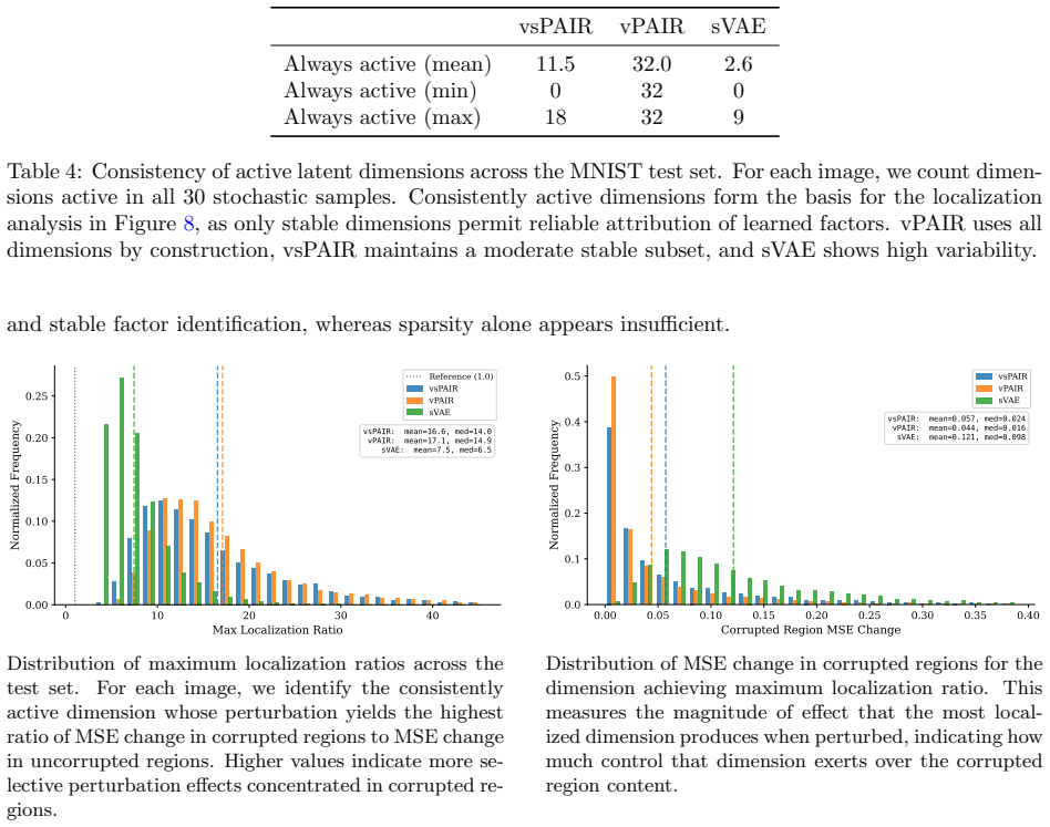
The central claim is that sparsity plus paired structure yields latent representations whose individual dimensions act as identifiable factors of uncertainty: a single dimension can be found that, when perturbed, disproportionately changes the reconstruction inside a corrupted region while leaving the image identity intact. On MNIST blind inpainting, the median maximum localization ratio is about 14 for vsPAIR, compared to about 6.5 for an unpaired sparse VAE, and the effect is not explained by the pool of stable dimensions. The paper argues this is because the QoI encoder is anchored to clean data, while a separate observation encoder and latent mapping keep the corruption from entangling t
Load-bearing premise
The load-bearing premise is that the learned latent dimensions remain stable, meaningful factors after training, so that the uncertainty-localized dimensions observed in one trained model reflect reusable structure rather than artifacts of one optimization run.
Editorial extensions
If this is right
- After training, inversion and uncertainty quantification require only three forward passes (encode y, map parameters, decode samples), making posterior sampling far cheaper than diffusion-based or iterative methods.
- The spike-and-slab latent separates two kinds of uncertainty: gating uncertainty (whether a factor is present) and slab uncertainty (what value the factor takes), which a dense VAE cannot express.
- On high-noise CT, vsPAIR outperforms learned primal-dual reconstruction in the paper's comparison and, unlike LPD or FBP, needs no access to the forward operator.
- The theoretical results show that in a linear-Gaussian setting, the learned parameter mapping is not just a heuristic: it provably produces samples from the correct conditional latent distribution.
- The paired structure, not sparsity alone, is what creates uncertainty-localized dimensions: on MNIST, vsPAIR's median maximum localization ratio is about 14 versus about 6.5 for an unpaired sparse VAE.
Reading between the lines
- If the localization effect survives retraining with different random seeds, the perturbation protocol could be used as a practical tool in medical imaging — a clinician could ask which latent factor, if changed, would alter the reconstruction in a region of interest.
- The localization ratio introduced here could become a standard metric for 'structured' UQ in inverse problems, complementing marginal calibration and giving interpretability a quantitative definition.
- The theorem's affine-encoder assumption points to a natural extension: replacing the linear mean map with a normalizing flow or a score-based encoder could bring the exactness guarantee closer to the CNN encoders used in practice.
- A testable extension would be to apply the same perturbation analysis to other forward operators (e.g., deblurring or super-resolution) and check whether the learned dimensions correspond to physically meaningful factors such as edges or textures rather than dataset-specific artifacts.
Editorial analysis
A structured set of objections, weighed in public.
Referee Report
Summary. The paper proposes vsPAIR, a paired-autoencoder architecture for inverse problems in which observations are encoded by a standard VAE and quantities of interest (QoI) by a sparse spike-and-slab VAE, with a learned mapping from observation latent parameters to QoI latent parameters. The framework is intended to provide fast amortized reconstruction together with interpretable, structured uncertainty quantification. The authors provide two theorems intended to justify the latent-mapping objective in a reduced Gaussian/linear setting, and report experiments on MNIST blind inpainting (comparing PAIR, vPAIR, sVAE, and vsPAIR) and on LoDoPaB-CT (comparing vsPAIR with FBP and Learned Primal-Dual). The central empirical evidence for structured uncertainty is a perturbation analysis in which latent dimensions are ranked by a 'localization ratio' measuring whether perturbation effects concentrate in corrupted versus uncorrupted image regions.
Significance. If the central claim is established, vsPAIR would be a valuable addition to the growing literature on amortized UQ for inverse problems: it combines fast inference, sparse interpretable latents, and a concrete way to trace uncertainty to image regions. The paper has notable strengths: a clean ablation design (PAIR vs vPAIR vs sVAE vs vsPAIR), extensive architecture and hyperparameter details, and candid acknowledgment of limitations. The theoretical results, however, are presented as only motivational, and the main empirical evidence for 'structured UQ' — the max-localization-ratio statistic — is currently not backed by a proper null model. The CT comparison supporting 'competitive reconstruction' is also not quantitatively controlled. These issues are fixable but are load-bearing for the paper's headline claims.
major comments (3)
- [§4.1, Figure 8 and Tables 4–5] The reported 'max localization ratio' is an order statistic. Under a null model in which perturbation effects on corrupted and uncorrupted pixels have comparable variability, the maximum over N candidate dimensions increases with N. The methods have very different N: vPAIR has 32 consistently active dimensions, vsPAIR about 11.5, and sVAE about 2.6; when 'all dimensions' are used, the sparse methods search 784 dimensions while vPAIR searches 32. Thus the medians (14.0, 14.9, 6.5) cannot be read directly as per-dimension selectivity. No permutation null, random-subset baseline, or per-dimension ratio distribution is provided. This is load-bearing because the central claim is precisely that paired sparsity yields latent dimensions that selectively target corrupted regions. I recommend reporting the full distribution of per-dimension localization ratios and comparing each method's observed
- [§3.2, Theorem 2] Theorem 2 as stated is not proven. The proof shows that p(y|z_x) is Gaussian as a function of y, but to conclude that p(z_x|y) is Gaussian as a function of z_x one needs the decoder mean μ_θ(z_x) to be affine in z_x. With a general Gaussian decoder, p(y|z_x) ∝ exp(−½(y − Aμ_θ(z_x))^T (A A^T + Σ_ε)^{-1}(y − Aμ_θ(z_x))), which is not quadratic in z_x unless μ_θ is affine; the product with the Gaussian prior is then not Gaussian. The missing affine-decoder assumption should be added, or the theorem should be revised. Relatedly, Theorem 1 assumes conditional independence and an affine/constant encoder map, neither of which holds for the jointly trained CNN and spike-and-slab encoders used in the experiments. The paper already calls these assumptions restrictive, but the language in the text should not give the impression that Theorems 1–2 support the empirical structured-UQ claims made later
- [§4.2, Figure 9 and surrounding text] The claim that vsPAIR outperforms LPD at high Gaussian noise levels is based on selected example slices; no aggregate PSNR/SSIM over the 800 test images or error bars are reported. The comparison is also not controlled: LPD has approximately 251k parameters and was trained for 500 epochs, while vsPAIR has approximately 1.1B parameters and was trained for 100 epochs. This makes the visual comparison difficult to interpret. Please provide aggregate metrics, uncertainty intervals, and either matched computational budgets or an explicit statement that the comparison is illustrative rather than a systematic benchmark.
minor comments (5)
- [Abstract] The abstract mentions 'initial-condition inference for the heat equation,' but the paper contains no heat-equation experiments. The abstract should be aligned with the actual content (MNIST inpainting and CT).
- [§4.1, Figure 5 and Figure 6] The notation '−400%', '−200%', '+200%', '+400%' for perturbations is unclear. Is the perturbation additive or multiplicative relative to the original latent value? A one-sentence definition in the text or caption would resolve the ambiguity.
- [Table 5] The rows labeled 'All dimensions' still do not compare like with like, because the number of searched dimensions differs (32 for vPAIR versus 784 for the sparse methods). A permutation null is needed even for these rows. Please state this explicitly or restrict the comparison to matched-size random subsets.
- [§4.2] The CT UQ analysis is qualitative and based on a small number of example slices. The authors acknowledge this in the discussion, but the text would benefit from a sentence in Section 4.2 explicitly stating that no quantitative UQ evaluation (e.g., calibration or region-based variance statistics) is attempted in the CT setting.
- [General] The paper states that code 'will be made available on Github upon initial acceptance.' Please include a versioned repository link or at least a release date; this is important for reproducibility of the perturbation and localization analyses.
Circularity Check
No circularity found: the learned latent mapping is an honest approximation target, the theoretical results are standard laws under stated assumptions, and self-citations are background rather than load-bearing.
full rationale
vsPAIR's core derivation is not circular. The latent mapping M← is trained by MSE to match the QoI encoder's own outputs (µx,Σx,ωx) on paired data (Eq. 16), and posterior sampling then draws from the mapped distribution (Sec. 3.1). This is an amortized approximation of the learned-encoder posterior, and the paper explicitly distinguishes that object from the true posterior p(x|y): 'this analysis concerns the posterior induced by the learned encoders, not the true data posterior' (Sec. 3.2). Theorems 1–2 follow from the tower property, the law of total covariance, and Gaussian marginalization under explicitly stated simplifying assumptions; they do not assume the conclusion about the actual CNN/spike-and-slab model. The sparse-UQ claims are empirical: localization ratios and perturbation effects are computed on held-out test images from the trained model, not from a parameter fitted to those same quantities. The main statistical concern is max-selection over different numbers of tested dimensions in Fig. 8 / Tables 4–5, which can bias the reported medians, but this is a correctness/interpretation issue rather than a definitional reduction; the paper partially addresses it by also searching over all dimensions. Self-citations to prior PAIR/latent-twin work supply background and training choices, but no load-bearing uniqueness theorem or ansatz is imported from them. No circular step is exhibited, so the appropriate score is 0.
Assumptions & free parameters
free parameters (5)
- Beta hyperprior parameters (α0, β0) =
MNIST (1,127); CT high-fidelity (502,1); CT UQ (1,64)
- Loss weights λ1, λ2, λ3, λρ, γx, γy, λb =
MNIST: 1,0.5,1,1.4,1.0,0.1,0.05; CT: 1,0.1,1,1.0,1e-4,1e-4,0
- Prior sparsity ρ (learned) =
≈0.05 active in MNIST (39/784 nnz); ≈0.86 active in CT UQ (7041/8192 nnz)
- Latent dimensionalities (ℓx, ℓy) =
MNIST (784,32); CT (8192,2048)
- Bernoulli temperature c =
50 (MNIST)
assumptions (6)
- domain assumption Assumption 1: E[X|Y=y] and Cov(X|Y=y) are continuous in y
- domain assumption Assumption 2: Z_x is conditionally independent of Y given X
- ad hoc to paper Assumption 3: μx(x)=Bx+c is affine and Σx(x) is constant
- ad hoc to paper Theorem 2 setting: Y=AX+ε with Gaussian ε, Gaussian decoder qθx(x|z_x), Gaussian p(z_x)
- standard math Universal Approximation Theorem for sufficiently expressive networks
- standard math sVAE spike-and-slab KL divergence formula from Tonolini et al. [37]
Cite this review
Pith. "Pith review of Variational Sparse Paired Autoencoders (vsPAIR) for Inverse Problems and Uncertainty Quantification." pith.science (2026). https://pith.science/paper/3V3RBUK6
@misc{pith2026260202948,
  author       = {Pith},
  title        = {Pith review of: Variational Sparse Paired Autoencoders (vsPAIR) for Inverse Problems and Uncertainty Quantification},
  year         = {2026},
  howpublished = {\url{https://pith.science/paper/3V3RBUK6}},
  note         = {Machine review of arXiv:2602.02948}
}
read the original abstract
Inverse problems are fundamental to many scientific and engineering disciplines; they arise when one seeks to reconstruct hidden, underlying quantities from noisy measurements. Many applications demand not just point estimates but interpretable uncertainty. Providing fast inference alongside uncertainty estimates remains challenging yet desirable in numerous applications. We propose the Variational Sparse Paired Autoencoder (vsPAIR) to address this challenge. The architecture pairs a standard VAE encoding observations with a sparse VAE encoding quantities of interest (QoI), connected through a learned latent mapping. The variational structure enables uncertainty estimation, the paired architecture encourages interpretability by anchoring QoI representations to clean data, and sparse encodings provide structure by concentrating information into identifiable factors rather than diffusing across all dimensions. To validate the effectiveness of our proposed architecture, we conduct experiments on blind inpainting, computed tomography (CT), and initial-condition inference for the heat equation, demonstrating that vsPAIR is a capable inverse problem solver that can provide interpretable and structured uncertainty estimates.
Figures


Figures from the paper (9 more)




Reference graph
Works this paper leans on
-
[1]
Jacques Hadamard.Lectures on Cauchy’s problem in linear partial differential equations. Vol. 15. Yale university press, 1923
1923
-
[2]
SIAM, 2002
Curtis R Vogel.Computational methods for inverse problems. SIAM, 2002
2002
-
[3]
SIAM, 2010
Per Christian Hansen.Discrete Inverse Problems: Insight and Algorithms. SIAM, 2010
2010
-
[4]
Daniela Calvetti and Erkki Somersalo.An introduction to Bayesian scientific computing: ten lectures on subjective computing. Vol. 2. Springer Science & Business Media, 2007
2007
-
[5]
Deep convolutional neural network for inverse problems in imaging
Kyong Hwan Jin et al. “Deep convolutional neural network for inverse problems in imaging”. In:IEEE Transactions on Image Processing26.9 (2017), pp. 4509–4522
2017
-
[6]
Image reconstruction by domain-transform manifold learning
Bo Zhu et al. “Image reconstruction by domain-transform manifold learning”. In:Nature555.7697 (2018), pp. 487–492. 23
2018
-
[7]
Plug-and-play priors for model based reconstruction
Singanallur V Venkatakrishnan, Charles A Bouman, and Brendt Wohlberg. “Plug-and-play priors for model based reconstruction”. In:IEEE Global Conference on Signal and Information Processing. IEEE. 2013, pp. 945–948
2013
-
[8]
The little engine that could: Regularization by denoising (RED)
Yaniv Romano, Michael Elad, and Peyman Milanfar. “The little engine that could: Regularization by denoising (RED)”. In:SIAM Journal on Imaging Sciences10.4 (2017), pp. 1804–1844
2017
Show all 79 references
-
[9]
Learning regularization functionals—a supervised training approach
E Haber and L Tenorio. “Learning regularization functionals—a supervised training approach”. In: Inverse Problems19.3 (Apr. 2003), p. 611.doi:10 . 1088 / 0266 - 5611 / 19 / 3 / 309.url:https : //doi.org/10.1088/0266-5611/19/3/309
2003 doi
-
[10]
Sebastian Lunz, Ozan ¨Oktem, and Carola-Bibiane Sch¨ onlieb.Adversarial Regularizers in Inverse Prob- lems. 2019. arXiv:1805.11572 [cs.CV].url:https://arxiv.org/abs/1805.11572
2019 arXiv
-
[11]
Learned Primal-Dual Reconstruction
Jonas Adler and Ozan Oktem. “Learned Primal-Dual Reconstruction”. In:IEEE Transactions on Medical Imaging37.6 (June 2018), pp. 1322–1332.issn: 1558-254X.doi:10.1109/tmi.2018.2799231. url:http://dx.doi.org/10.1109/TMI.2018.2799231
2018
-
[12]
Algorithm unrolling: Interpretable, efficient deep learning for signal and image processing
Vishal Monga, Yuelong Li, and Yonina C Eldar. “Algorithm unrolling: Interpretable, efficient deep learning for signal and image processing”. In:IEEE Signal Processing Magazine38.2 (2021), pp. 18– 44
2021
-
[13]
Good Things Come in Pairs: Paired Autoencoders for Inverse Problems
Matthias Chung, Bas Peters, and Michael Solomon. “Good Things Come in Pairs: Paired Autoencoders for Inverse Problems”. In:arXiv preprint arXiv:2505.06549(2025)
2025 arXiv
-
[14]
Auto-encoding variational bayes
Diederik P Kingma and Max Welling. “Auto-encoding variational bayes”. In:arXiv preprint arXiv:1312.6114 (2013)
2013 arXiv
-
[15]
Reducing the dimensionality of data with neural networks
Geoffrey E Hinton and Ruslan R Salakhutdinov. “Reducing the dimensionality of data with neural networks”. In:Science313.5786 (2006), pp. 504–507
2006
-
[16]
Stacked Denoising Autoencoders: Learning Useful Representations in a Deep Network with a Local Denoising Criterion
Pascal Vincent et al. “Stacked Denoising Autoencoders: Learning Useful Representations in a Deep Network with a Local Denoising Criterion”. In:Journal of Machine Learning Research11.110 (2010), pp. 3371–3408.url:http://jmlr.org/papers/v11/vincent10a.html
2010
-
[17]
Yoshua Bengio et al.Generalized Denoising Auto-Encoders as Generative Models. 2013. arXiv:1305. 6663 [cs.LG].url:https://arxiv.org/abs/1305.6663
2013 arXiv
-
[18]
Variational Autoencoder Inverse Mapper: An End-to-End Deep Learning Frame- work for Inverse Problems
Manal Almaeen et al. “Variational Autoencoder Inverse Mapper: An End-to-End Deep Learning Frame- work for Inverse Problems”. In:2021 International Joint Conference on Neural Networks (IJCNN). 2021, pp. 1–8.doi:10.1109/IJCNN52387.2021.9534012
2021
-
[19]
Housen Li et al.NETT: Solving Inverse Problems with Deep Neural Networks. 2019. arXiv:1803.00092 [math.NA].url:https://arxiv.org/abs/1803.00092
2019 arXiv
-
[20]
Paired autoencoders for likelihood-free estimation in inverse problems
Matthias Chung et al. “Paired autoencoders for likelihood-free estimation in inverse problems”. In: Machine Learning: Science and Technology5.4 (2024), p. 045055
2024
-
[21]
A paired autoencoder framework for inverse problems via bayes risk minimization
Emma Hart, Julianne Chung, and Matthias Chung. “A paired autoencoder framework for inverse problems via bayes risk minimization”. In:arXiv preprint arXiv:2501.14636(2025)
2025 arXiv
-
[22]
Latent Twins
Matthias Chung et al. “Latent Twins”. In:arXiv preprint arXiv:2509.20615(2025)
2025
-
[23]
Diffusion posterior sampling for general noisy inverse problems
Hyungjin Chung et al. “Diffusion posterior sampling for general noisy inverse problems”. In:Interna- tional Conference on Learning Representations. 2023
2023
-
[24]
Solving inverse problems in medical imaging with score-based generative models
Yang Song et al. “Solving inverse problems in medical imaging with score-based generative models”. In:International Conference on Learning Representations. 2022
2022
-
[25]
Denoising diffusion restoration models
Bahjat Kawar et al. “Denoising diffusion restoration models”. In:Advances in Neural Information Processing Systems. Vol. 35. 2022, pp. 23593–23606
2022
-
[26]
Richard Durrett.Probability: theory and examples. Second. Belmont, CA: Duxbury Press, 1996.isbn: 0-534-24318-5. 24
1996
-
[27]
Inverse problems: a Bayesian perspective
Andrew M Stuart. “Inverse problems: a Bayesian perspective”. In:Acta numerica19 (2010), pp. 451– 559
2010
-
[28]
The restricted isometry property and its implications for compressed sensing
Emmanuel J Candes. “The restricted isometry property and its implications for compressed sensing”. In:Comptes rendus. Mathematique346.9-10 (2008), pp. 589–592
2008
-
[29]
A variable projection method for large-scale inverse prob- lems with l1 regularization
Matthias Chung and Rosemary A Renaut. “A variable projection method for large-scale inverse prob- lems with l1 regularization”. In:Applied Numerical Mathematics192 (2023), pp. 297–318
2023
-
[30]
Fast L1-regularized EEG source localization using variable projection
Jack Michael Solomon, Rosemary Anne Renaut, and Matthias Chung. “Fast L1-regularized EEG source localization using variable projection”. In:Inverse Problems41.6 (2025), p. 065014
2025
-
[31]
Christopher KI Williams and Carl Edward Rasmussen.Gaussian processes for machine learning. Vol. 2
-
[32]
MIT press Cambridge, MA, 2006
2006
-
[33]
Multilayer feedforward networks are universal approximators
Kurt Hornik, Maxwell Stinchcombe, and Halbert White. “Multilayer feedforward networks are universal approximators”. In:Neural networks2.5 (1989), pp. 359–366
1989
-
[34]
SPARSE L1-AUTOENCODERS FOR SCIENTIFIC DATA COMPRESSION
Matthias Chung et al. “SPARSE L1-AUTOENCODERS FOR SCIENTIFIC DATA COMPRESSION”. In:Journal of Machine Learning for Modeling and Computing6.4 (2025), pp. 51–71.issn: 2689-3967
2025
-
[35]
Murphy.Probabilistic Machine Learning: An introduction
Kevin P. Murphy.Probabilistic Machine Learning: An introduction. MIT Press, 2022.url:http : //probml.github.io/book1
2022
-
[36]
An Introduction to Variational Autoencoders
Diederik P Kingma and Max Welling. “An Introduction to Variational Autoencoders”. In:Foundations and Trends in Machine Learning12.4 (2019), pp. 307–392
2019
-
[37]
Fixing a Broken ELBO
Alexander A Alemi et al. “Fixing a Broken ELBO”. In:International Conference on Machine Learning. PMLR. 2018, pp. 159–168
2018
-
[38]
Variational Sparse Coding
Francesco Tonolini, Bjørn Sand Jensen, and Roderick Murray-Smith. “Variational Sparse Coding”. In: Proceedings of The 35th Uncertainty in Artificial Intelligence Conference. PMLR, Aug. 2020, pp. 690–
2020
-
[39]
Boink and Christoph Brune.Learned SVD: solving inverse problems via hybrid autoencoding
Yoeri E. Boink and Christoph Brune.Learned SVD: solving inverse problems via hybrid autoencoding
-
[40]
Bayesian Variable Selection in Linear Regression
Toby J. Mitchell and John J. Beauchamp. “Bayesian Variable Selection in Linear Regression”. In: Journal of the American Statistical Association83.404 (1988), pp. 1023–1032.doi:10.1080/01621459. 1988.10478694
1988
-
[41]
Ilya Tolstikhin et al.Wasserstein Auto-Encoders. 2019. arXiv:1711.01558 [stat.ML].url:https: //arxiv.org/abs/1711.01558
2019 arXiv
-
[42]
Flow-Based Models
Jakub M. Tomczak. “Flow-Based Models”. In:Deep Generative Modeling. Cham: Springer Interna- tional Publishing, 2024, pp. 63–92.isbn: 978-3-031-64087-2.doi:10.1007/978- 3- 031- 64087- 2_4. url:https://doi.org/10.1007/978-3-031-64087-2_4
2024 doi
-
[43]
Moritz Piening and Matthias Chung.Paired Wasserstein Autoencoders for Conditional Sampling. 2024. arXiv:2412.07586 [cs.LG].url:https://arxiv.org/abs/2412.07586
2024
-
[44]
Multilayer feedforward networks are universal approximators
Kurt Hornik, Maxwell Stinchcombe, and Halbert White. “Multilayer feedforward networks are universal approximators”. In:Neural Networks2.5 (1989), pp. 359–366.issn: 0893-6080.doi:https://doi. org/10.1016/0893-6080(89)90020-8.url:https://www.sciencedirect.com/science/article/ pi...
1989
-
[45]
LoDoPaB-CT, a benchmark dataset for low-dose computed tomography reconstruction
Johannes Leuschner et al. “LoDoPaB-CT, a benchmark dataset for low-dose computed tomography reconstruction”. In:Scientific Data8.1 (Apr. 2021).issn: 2052-4463.doi:10 . 1038 / s41597 - 021 - 00893-z.url:http://dx.doi.org/10.1038/s41597-021-00893-z. 25
2021 doi
-
[46]
Blitzstein and Jessica Hwang.Introduction to Probability Second Edition
Joseph K. Blitzstein and Jessica Hwang.Introduction to Probability Second Edition. Taylor and Francis Group, 2019
2019
-
[47]
Chapter 6: Filtered Back-Projection
J. S. Jørgensen and W. R. B. Lionheart. “Chapter 6: Filtered Back-Projection”. In:Computed Tomogra- phy: Algorithms, Insight, and Just Enough Theory, pp. 73–103.doi:10.1137/1.9781611976670.ch6. eprint:https://epubs.siam.org/doi/pdf/10.1137/1.9781611976670.ch6.url:https://epubs...
-
[48]
com / cetmann / pytorch - primaldual
Christian Etmann.pytorch-primaldual.https : / / github . com / cetmann / pytorch - primaldual. GitHub repository. 2020
2020
-
[49]
The Lung Image Database Consortium (LIDC) and Image Database Resource Initiative (IDRI): a completed reference database of lung nodules on CT scans
Samuel G. Armato III et al. “The Lung Image Database Consortium (LIDC) and Image Database Resource Initiative (IDRI): a completed reference database of lung nodules on CT scans”. In:Medical Physics38.2 (Feb. 2011), pp. 915–931.issn: 0094-2405.doi:10 . 1118 / 1 . 3528204.url:ht...
2011
-
[50]
Dongsoo Lee et al.Learning Low-Rank Approximation for CNNs. 2019. arXiv:1905.10145 [cs.LG]. url:https://arxiv.org/abs/1905.10145
2019 arXiv
-
[51]
A review of uncertainty quantification in medical image analysis: Probabilistic and non-probabilistic methods
Ling Huang et al. “A review of uncertainty quantification in medical image analysis: Probabilistic and non-probabilistic methods”. In:Medical Image Analysis97 (2024), p. 103223
2024
-
[52]
Alireza Azadbakht et al.Drastically Reducing the Number of Trainable Parameters in Deep CNNs by Inter-layer Kernel-sharing. 2022. arXiv:2210.14151 [cs.CV].url:https://arxiv.org/abs/2210. 14151
2022 arXiv
-
[53]
Uncertainty quantification in time-lapse seismic imaging: a full-waveform approach
Maria Kotsi, Alison Malcolm, and Gregory Ely. “Uncertainty quantification in time-lapse seismic imaging: a full-waveform approach”. In:Geophysical Journal International222.2 (2020), pp. 1245– 1263
2020
-
[54]
Tomczak and Max Welling.V AE with a VampPrior
Jakub M. Tomczak and Max Welling.V AE with a VampPrior. 2018. arXiv:1705.07120 [cs.LG].url: https://arxiv.org/abs/1705.07120
2018 arXiv
-
[55]
A review of uncertainty quantification in deep learning: Techniques, applications and challenges
Moloud Abdar et al. “A review of uncertainty quantification in deep learning: Techniques, applications and challenges”. In:Information Fusion76 (2021), pp. 243–297
2021
-
[56]
Multi-task Sparse Learning with Beta Process Prior for Action Recognition
Chunfeng Yuan et al. “Multi-task Sparse Learning with Beta Process Prior for Action Recognition”. In:2013 IEEE Conference on Computer Vision and Pattern Recognition. 2013, pp. 423–429.doi: 10.1109/CVPR.2013.61
2013 doi
-
[57]
Victor Prokhorov et al.Learning Sparse Sentence Encoding without Supervision: An Exploration of Sparsity in Variational Autoencoders. 2021. arXiv:2009.12421 [cs.CL].url:https://arxiv.org/ abs/2009.12421
2021 arXiv
-
[58]
Shakir Mohamed, Katherine Heller, and Zoubin Ghahramani.Bayesian and L1 Approaches to Sparse Unsupervised Learning. 2012. arXiv:1106.1157 [cs.LG].url:https://arxiv.org/abs/1106.1157
2012 arXiv
-
[59]
Yoshua Bengio, Nicholas L´ eonard, and Aaron Courville.Estimating or Propagating Gradients Through Stochastic Neurons for Conditional Computation. 2013. arXiv:1308 . 3432 [cs.LG].url:https : //arxiv.org/abs/1308.3432
2013 arXiv
-
[60]
Maddison, Andriy Mnih, and Yee Whye Teh.The Concrete Distribution: A Continuous Re- laxation of Discrete Random Variables
Chris J. Maddison, Andriy Mnih, and Yee Whye Teh.The Concrete Distribution: A Continuous Re- laxation of Discrete Random Variables. 2017. arXiv:1611.00712 [cs.LG].url:https://arxiv.org/ abs/1611.00712
2017 arXiv
-
[61]
Learning sparse neural networks through L0 regularization
Christos Louizos, Max Welling, and Diederik P Kingma. “Learning sparse neural networks through L0 regularization”. In:arXiv preprint arXiv:1712.01312(2017)
2017 arXiv
-
[62]
Rozell.Variational Sparse Coding with Learned Thresholding
Kion Fallah and Christopher J. Rozell.Variational Sparse Coding with Learned Thresholding. 2022. arXiv:2205.03665 [cs.LG].url:https://arxiv.org/abs/2205.03665
2022 arXiv
-
[63]
Aaron van den Oord, Oriol Vinyals, and Koray Kavukcuoglu.Neural Discrete Representation Learning
-
[64]
Jason Tyler Rolfe.Discrete Variational Autoencoders. 2017. arXiv:1609 . 02200 [stat.ML].url: https://arxiv.org/abs/1609.02200
2017 arXiv
-
[65]
Yarman-Vural.L-V AE: Variational Auto-Encoder with Learnable Beta for Disentangled Representation
Hazal Mogultay Ozcan, Sinan Kalkan, and Fatos T. Yarman-Vural.L-V AE: Variational Auto-Encoder with Learnable Beta for Disentangled Representation. 2025. arXiv:2507.02619 [cs.LG].url:https: //arxiv.org/abs/2507.02619
2025 arXiv
-
[66]
Challenging Common Assumptions in the Unsupervised Learning of Dis- entangled Representations
Francesco Locatello et al. “Challenging Common Assumptions in the Unsupervised Learning of Dis- entangled Representations”. In:Proceedings of the 36th International Conference on Machine Learn- ing. Ed. by Kamalika Chaudhuri and Ruslan Salakhutdinov. Vol. 97. Proceedings of Ma...
2019
-
[67]
Bishop.Pattern Recognition and Machine Learning (Information Science and Statis- tics)
Christopher M. Bishop.Pattern Recognition and Machine Learning (Information Science and Statis- tics). Berlin, Heidelberg: Springer-Verlag, 2006.isbn: 0387310738
2006
-
[68]
Burgess et al.Understanding disentangling inβ-V AE
Christopher P. Burgess et al.Understanding disentangling inβ-V AE. 2018. arXiv:1804.03599 [stat.ML]. url:https://arxiv.org/abs/1804.03599
2018 arXiv
-
[69]
Kingma and Jimmy Ba.Adam: A Method for Stochastic Optimization
Diederik P. Kingma and Jimmy Ba.Adam: A Method for Stochastic Optimization. 2017. arXiv:1412. 6980 [cs.LG].url:https://arxiv.org/abs/1412.6980. A sV AE Implementation Details Beta Hyperprior for Adaptive Sparsity .Introducing sparsity into an sV AE is not trivial and a sparsit...
2017 arXiv
-
[72]
Robert.Bayesian Essentials with R
Jean-Michel Marin and Christian P. Robert.Bayesian Essentials with R. Springer Texts in Statistics. New York, NY: Springer New York, 2014.isbn: 978-1-4614-8686-2.doi:10.1007/978-1-4614-8687-9. url:http://link.springer.com/10.1007/978-1-4614-8687-9(visited on 07/01/2021)
2014 doi
-
[74]
This motivates structure in the latent representations
originally leveraged a classifier-based approach that builds off of [54], where a classifier is used to pick a specific prior for each input, based on trained pseudo-inputs. This motivates structure in the latent representations. For simplicity, we fix the prior level of spars...
-
[75]
Sample uniform noiseη i ∼Uniform(0,1)
-
[76]
Compute a relaxation of the thresholding via the differentiable step function approximation:s i = σ c(ηi −1 +ω i) ∈(0,1), wherec >0 is a temperature parameter ([37, 60])
-
[77]
Threshold to obtain exact zeros: ˆs i =1 {si>0.5}(si)∈ {0,1}
-
[78]
Straight-through gradient estimation: construct a mask, mask i, using the thresholded values, but use the gradient ofs i for backpropagation [59, 62, 63]
-
[79]
B Hyperparameter Selection The vsPAIR framework requires tuning several hyperparameters for training
Apply the standard reparameterizationz ∗ i =µ i +σ iϵi withϵ i ∼ N(ϵ|0,1), then mask:z i = maski ·z ∗ i [14]. B Hyperparameter Selection The vsPAIR framework requires tuning several hyperparameters for training. Parameter estimation for scientific machine learning is an extens...
-
[700]
(Visited on 11/11/2024)
2024
-
[2018]
arXiv:1711.00937 [cs.LG].url:https://arxiv.org/abs/1711.00937. 26
-
[2020]
arXiv:1912.10840 [cs.LG].url:https://arxiv.org/abs/1912.10840
1912 arXiv
Reviewed August 3, 2026 · model on record in the stance chip above.
Discussion (0). Sign in to comment.