REVIEW 3 major objections 4 minor 1 cited by
Comparison of Structure Preserving Schemes for the Cahn-Hilliard-Navier-Stokes Equations with Degenerate Mobility and Adaptive Mesh Refinement
T0 review · 3 major / 4 minor · reviewed 2026-08-03 · deepseek-v4-flash
Pith's one-line read This paper establishes that, for the Cahn–Hilliard–Navier–Stokes system with degenerate mobility, an element-wise scaling limiter applied to discontinuous Galerkin or finite element discretizations yields schemes that simultaneously conserv
desk verdict Useful benchmark comparison and two new scheme variants, but the energy-dissipation theorem ignores the advection term and should be fixed before the paper is treated as a theoretical reference. read the letter →
The pith
A machine-rendered reading of the paper's core claim, the machinery that carries it, and where it could break.
The reading
What carries the argument
The element-wise scaling limiter: on each element K, the phase-field polynomial ψ_h is scaled around its cell mean ψ̄_K by a factor α_K chosen so that all quadrature points lie within [ψ_min, ψ_max]=[−1, 1]. Because the cell mean is unchanged, the limiter is mass-conservative by construction, and it enforces the bound provided the cell averages are already inside the interval. Supporting this, the paper proves coercivity of a weighted interior-penalty bilinear form; the harmonic-average weighting (SWIP) is the key modification that lowers the mobility contrast and improves conditioning of the linear systems.
What would settle it
Run the SWIP-L scheme on a coarse adaptive mesh with a strong advection field, starting from initial data with cell averages inside [−1, 1], and check whether any pre-limiter cell average exits [−1, 1] after the first IMEX step. If it does, the scaling limiter in Eq. (83) cannot restore the bound and the boundedness claim fails. Alternatively, test whether the discrete energy in Eq. (67) is monotonically non-increasing for a range of penalty parameters; a violation would contradict Theorem 3.3.
Extended reading notes
Core claim
The central claim is that structure preservation for the CHNS system with degenerate mobility M(ψ)=1−ψ² is achievable without sacrificing accuracy or mass conservation. Applying an element-wise scaling limiter to either DG (SIPG/SWIP) or standard FEM discretizations yields schemes that conserve phase-field mass, keep the phase field in [−1, 1], and dissipate the discrete free energy in every test performed. The paper further claims that the proposed SWIP variant, which weights the numerical fluxes using harmonic averages of the degenerate mobility, reduces the mobility contrast over element faces, leading to a better-conditioned and more reliable scheme than standard SIPG while preserving th
Load-bearing premise
The scaling limiter can only enforce ψ∈[−1, 1] if the cell average of the computed phase-field already lies in [−1, 1]; the paper assumes, based on numerical observation but without a discrete proof, that the degenerate-mobility scheme keeps cell averages in bounds.
Editorial extensions
If this is right
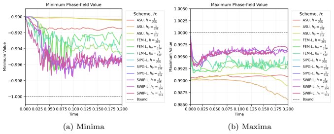
- The limited schemes FEM-L, SIPG-L, and SWIP-L, together with the ASU scheme, achieve all three structure-preserving properties (mass conservation, bound preservation, energy dissipation) in every numerical test; unlimited FEM, SIPG, and SWIP violate the bounds.
- The scaling limiter avoids the O(10⁻⁴) mass loss of the cut-off method (FEM-C), so applications that need in-bounds phase fields can use the limited schemes instead of artificial post-processing.
- The DG schemes converge at O(h²) in L2 for piecewise-linear elements, while the ASU scheme converges at O(h); the DG schemes achieve comparable accuracy to FEM at coarser meshes, reducing computational time.
- The SWIP-L scheme is better conditioned than SIPG-L, making it the recommended choice among the DG variants, especially in combination with adaptive mesh refinement.
- The structure-preserving properties survive conforming adaptive mesh refinement with the indicator function (1−ψ_h²)⁴, which focuses refinement at the interface.
Reading between the lines
- The discrete bound-preservation theorem is conditional: it holds only if the cell average of the un-limited phase-field lies in [−1, 1]. A rigorous proof for the regularized degenerate-mobility scheme would close the gap the paper leaves open.
- The harmonic-average weighting idea could transfer to other degenerate-mobility or strongly heterogeneous diffusion problems, where face-averaged coefficients create large contrast and degrade conditioning.
- The mass drift observed for FEM-L in the coupled CHNS tests may stem from the interaction between the limiter and the non-divergence-free Taylor–Hood velocity field; a divergence-free velocity discretization might remove this drift.
- A systematic parameter sweep in the penalty parameter η and mobility regularization δ could map the actual coercivity margin of SWIP and reveal when the scheme ceases to be energy dissipative.
Editorial analysis
A structured set of objections, weighed in public.
Referee Report
Summary. The paper presents a systematic numerical comparison of structure-preserving discretizations for the Cahn-Hilliard-Navier-Stokes (CHNS) system with degenerate mobility, in the setting of conforming adaptive mesh refinement. The schemes considered are continuous FEM (with and without a cut-off post-processing, with and without a scaling limiter), DG-SIPG and DG-SWIP (both with and without a scaling limiter), and the upwind ASU scheme. The authors provide a DG formulation with a weighted-SWIP variant and a scaling limiter, and they report convergence rates, mass conservation, phase-field boundedness, and energy dissipation for pure CH and coupled CHNS test cases, including a rising-bubble benchmark. The central recommendation is that only the limited schemes (FEM-L, SIPG-L, SWIP-L) and ASU preserve both mass and bounds, while the standard unlimited schemes violate the bounds and the cut-off FEM loses mass at O(10^-4). SWIP-L is highlighted as the most robust among the DG variants.
Significance. If the comparison and the associated software are reliable, this is a useful practical contribution: it gives a head-to-head assessment of recently proposed structure-preserving schemes in a UFL/Dune-Fem framework, with reproducible code, adaptive-mesh benchmarks, and a clear recommendation for users who need boundedness and mass conservation in multiphase flow simulations. The numerical study is carefully structured, with convergence-rate tables, mass/energy/bounds tables, and adaptive-grid experiments. The paper also explicitly acknowledges some open theoretical points (e.g., ASU energy dissipation in the decoupled CHNS setting, and the cell-average assumption for the limiter), which is a strength. However, the theoretical support for the energy-dissipation claims in the advective case is not correct as stated, and the boundedness proof for the limited schemes is explicitly conditional on an unproven cell-average property. These issues affect the interpretation of the headline claims, although the numerical evidence itself appears solid.
major comments (3)
- [§3.3, Theorem 3.3 and Eq. (68)] The claimed energy identity is not valid for the advective DG formulation. The phase-field equation in Eqs. (64)–(65) contains the discrete advection term −c(u,ψ_h,φ) from Eq. (63). Setting φ=υ_h in that equation gives ⟨∂tψ_h,υ_h⟩ = c(u,ψ_h,υ_h) − Pe^{-1} b(M(ψ_h),υ_h,υ_h). The energy derivative ∂tE[ψ_h] therefore contains the c-term, which does not vanish in general for the upwind DG discretization with a solenoidal u. The proof of Theorem 3.3 simply asserts the dissipation without deriving this identity, and Eq. (68) is not a consequence of the discrete scheme. In the continuous CHNS setting only the total energy (24), including the kinetic energy, is dissipated; the phase-field energy alone is not monotone under advection. Consequently, Theorem 3.3 cannot justify the 'energy dissipative' entries for the coupled runs in Table 5. The numerical energy plots in Sections 4.4–4.5 may well b
- [§3.5, Corollary 3.6.1 and Remark 3.12] The boundedness of FEM-L, SIPG-L, and SWIP-L is conditional on the cell averages of the phase-field remaining in [-1,1] after each time step. This is stated explicitly in Corollary 3.6.1 ('provided that the FEM phase-field for each element K satisfies 1/|K|∫_K ψ̃_h dx ∈ [-1,1]') and in Remark 3.12, where the authors say this condition is not proven and only 'no violation ... has been encountered' in the experiments. The scaling limiter in Eq. (83) scales around the mean value, so if the mean itself lies outside the interval the limiter cannot restore the bounds while preserving mass. Thus Table 5's 'boundedness' column for these schemes is not a proven structure-preservation property, only an observed one. Since boundedness is one of the three advertised structure-preserving properties and a central part of the paper's recommendation, this conditional should be prominently qualified in t
- [§3.2, Theorem 3.2 and Remark 3.3] The coercivity theorem requires the mobility-dependent penalty Λ_e(M(ψ_h)) to be at least of order λ⋆, the global contrast defined in Eq. (47), cf. Eq. (52). With the regularized mobility M_δ (the text uses δ=10^{-20} in §3.2 and δ=10^{-14} in the UFL code), the contrast λ⋆ can be very large near ψ=±1, since the denominator min_K M(ψ_h) is of order δ. However, Remark 3.3 fixes Λ_e=5 and η=k(k+d−1)(θ+1)^2/4 for all computations. These values do not in general satisfy the sufficient inequality (52) unless λ⋆ is bounded by a small mesh-independent constant, which is not established. The authors note the dependence on smoothness of ψ_h but do not verify it for their examples. This is not a fatal flaw for a numerical comparison, but the paper presents Theorem 3.2 as a theoretical foundation for the SWIP-L/SIPG-L schemes; the connection between the theorem and the actual computational paramete
minor comments (4)
- [Eq. (63)–(65)] Please check the sign convention of the advection form c(u,ψ_h,φ). Eq. (64) writes ⟨∂tψ_h,v⟩ − c(u,ψ_h,φ) + ..., while the continuous equation (17) contains +∇·(uψ). If c is defined by Eq. (63) as ∫_Th u·∇φ ψ_h dx − Σ(...)[φ]ds, then −c corresponds to the standard weak form only after an integration by parts; the sign conventions should be stated explicitly and made consistent in all formulae and UFL listings.
- [Eq. (67)] The DG energy lifting in Eq. (67) writes the last term as '−(1+θ){∇ψ_h·n+}[ψ]' without the surface measure ds. Please add the missing measure and check the boundary terms. Also clarify how this discrete energy relates to the continuous total energy (24) in the coupled CHNS runs shown in Figs. 12, 15, and 18.
- [Table 5 and Section 4.5.2] In Table 5 the footnote for FEM-L is not referenced or explained in the text. Also, in Section 4.5.2 the statement 'The simulations using Ex. 4.4 did not converge using the ASU scheme' is a notable negative result that is not discussed. A brief explanation (e.g., conditioning, coupling, or time-step restrictions) would help the reader interpret the comparison.
- [References [13] and [39]] Refs. [13] and [39] appear to be the same article (one published, one preprint), with the same DOI in the bibliography. Please consolidate the citations and avoid duplicate entries.
Circularity Check
No circularity: the paper's central claims are benchmark comparisons and explicitly conditional numerical observations; the flagged energy-theorem gap is a rigor issue, not a circular reduction.
full rationale
The derivation chain is not circular. The paper's theoretical results (coercivity of the SWIP/SIPG bilinear form, weak mass conservation, and the conditional bound-preservation statements) are standard DG/FEM arguments with explicit assumptions. Bound preservation for the limited schemes is honestly stated as conditional on the unproven cell-average condition (Remark 3.12 and Corollary 3.6.1), and the paper reports that no violation was observed; this is an assumption plus numerical evidence, not a fitted input relabeled as a prediction. The comparative claims in Tables 2 and 5 are numerical observations on external benchmark problems (e.g., the rising bubble benchmark), not parameters fitted to the data and then called predictions. Self-citations ([27], [28], [44], [50]) concern software infrastructure and limiter implementation, and are not load-bearing for the mathematical results. The main rigor problem is Theorem 3.3: the proof of Eq. (68) omits the advection term c(u, ψ_h, υ_h) from Eq. (63) that appears when the phase-field equation is tested with υ_h, and the coefficients in the discrete energy Eq. (67) do not match the physical energy Eq. (24). Consequently the energy-dissipation column of Table 5 is not established by the stated theorem. That is an omitted-proof/correctness issue, not a circularity: the energy identity is not assumed as an input, and energy decay is reported from simulations rather than derived from constituents that already contain the conclusion.
Assumptions & free parameters
free parameters (6)
- Penalty scaling Λ_e for DG interior-penalty terms =
5
- Mobility regularization floor δ =
1e-20 (theory), 1e-14 (SWIP UFL)
- Adaptivity thresholds =
refine H<0.0525, coarsen H>0.15
- Initial phase-field amplitude =
0.99
- Nonlinear solver tolerance ε =
1e-16 for most runs, 5e-16 for the bubble benchmark, 1e-12/1e-14/1e-16 in the tolerance study
- Cahn and Péclet settings Cn=4h, Pe^-1=3Cn =
Cn=4h or O(0.01), Pe^-1=3Cn
assumptions (7)
- standard math Trace and inverse inequalities of Lemma 3.1 hold on regular quadrilateral/triangular tessellations
- domain assumption The domain Ω is convex for the continuous bound-preservation theorem
- domain assumption The variable-density CHNS model of [8] is the correct physical model
- domain assumption The regularized mobility Mδ=max(M,δ) inherits the bound-preserving behavior of M
- ad hoc to paper Discrete cell averages of the phase-field remain in [-1,1] for the limited schemes
- ad hoc to paper The scaling limiter does not destroy energy dissipation
- ad hoc to paper ASU bound/mass-preservation proofs on uniform triangular grids extend to conformally adaptive triangular grids
Cite this review
Pith. "Pith review of Comparison of Structure Preserving Schemes for the Cahn-Hilliard-Navier-Stokes Equations with Degenerate Mobility and Adaptive Mesh Refinement." pith.science (2026). https://pith.science/paper/6SOENWOY
@misc{pith2026260208639,
  author       = {Pith},
  title        = {Pith review of: Comparison of Structure Preserving Schemes for the Cahn-Hilliard-Navier-Stokes Equations with Degenerate Mobility and Adaptive Mesh Refinement},
  year         = {2026},
  howpublished = {\url{https://pith.science/paper/6SOENWOY}},
  note         = {Machine review of arXiv:2602.08639}
}
read the original abstract
The Cahn-Hilliard-Navier-Stokes (CHNS) system utilizes a diffusive phase-field for interface tracking of multi-phase fluid flows. Recently structure preserving methods for CHNS have moved into focus to construct numerical schemes that, for example, are mass conservative or obey initial bounds of the phase-field variable. In this work decoupled implicit-explicit formulations based on the Discontinuous Galerkin (DG) methodology are considered and compared to existing schemes from the literature. For the fluid flow a standard continuous Galerkin approach is applied. An adaptive conforming grid is utilized to further draw computational focus on the interface regions, while coarser meshes are utilized around pure phases. All presented methods are compared against each other in terms of bound preservation, mass conservation, and energy dissipation for different examples found in the literature, including a classical rising droplet problem.
Figures


Figures from the paper (16 more)




Forward citations
Cited by 1 Pith paper
-
On $hp$-adaptive Structure-Preservion for the Cahn--Hilliard--Navier--Stokes Equations with Degenerate Mobility
New α-weighted mobility fluxes give DG schemes for degenerate-mobility Cahn-Hilliard-Navier-Stokes that are coercive under an unverified a-priori penalty bound, show optimal convergence in tests, and preserve energy, ...
Reference graph
Works this paper leans on
-
[1]
J. Cahn, J. Hilliard, Free Energy of a Nonuniform System. I. Interfacial Free Energy, The Journal of Chemical Physics 28 (2) (1958).doi:10. 1063/1.1744102
1958
-
[2]
Y. Pan, K. Suga, Numerical simulation of binary liquid droplet collision, Physics of Fluids 17 (8) (2005).doi:10.1063/1.2009527. 43
-
[3]
N. Nikolopoulos, K.-S. Nikas, G. Bergeles, A numerical investigation of central binary collision of droplets, Computers & Fluids 38 (6) (2009) 1191– 1202.doi:10.1016/j.compfluid.2008.11.007
-
[4]
P. C. Hohenberg, B. I. Halperin, Theory of dynamic critical phenomena, Rev. Mod. Phys. 49 (1977) 435–479.doi:10.1103/RevModPhys.49.435
-
[5]
D. Lee, J.-Y. Huh, D. Jeong, J. Shin, A. Yun, J. Kim, Physical, mathe- matical, and numerical derivations of the cahn–hilliard equation, Compu- tational Materials Science 81 (2014) 216–225.doi:10.1016/j.commatsci. 2013.08.027
-
[6]
M. F. P. ten Eikelder, K. G. van der Zee, I. Akkerman, D. Schillinger, A uni- fied framework for Navier-Stokes Cahn-Hilliard models with non-matching densities, Mathematical Models and Methods in Applied Sciences 33 (01) (2023) 175–221.doi:10.1142/S0218202523500069
-
[7]
J. S. Lowengrub, L. Truskinovsky, Quasi-incompressible Cahn-Hilliard flu- ids and topological transitions, Proceedings of the Royal Society of London. Series A: Mathematical, Physical and Engineering Sciences 454 (1998) 2617 – 2654.doi:10.1098/rspa.1998.0273
arXiv 1998
-
[8]
H. Abels, H. Garcke, G. Grün, Thermodynamically Consistent, Frame Indifferent Diffuse Interface Models For Incompressible Two-Phase Flows With Different Densities, Mathematical Models and Methods in Applied Sciences 22 (03) (2012) 1150013.doi:10.1142/S0218202511500138
Show all 57 references
-
[9]
Boyer, A theoretical and numerical model for the study of incompressible mixture flows, Computers & Fluids 31 (1) (2002) 41–68.doi:10.1016/ S0045-7930(00)00031-1
F. Boyer, A theoretical and numerical model for the study of incompressible mixture flows, Computers & Fluids 31 (1) (2002) 41–68.doi:10.1016/ S0045-7930(00)00031-1
2002
-
[10]
J. Shen, X. Yang, Numerical approximations of Allen-Cahn and Cahn- Hilliard equations (2010).doi:10.3934/dcds.2010.28.1669
2010 doi
-
[11]
H. Ding, P. D. Spelt, C. Shu, Diffuse interface model for incompressible two-phase flows with large density ratios, Journal of Computational Physics 226 (2) (2007) 2078–2095.doi:10.1016/j.jcp.2007.06.028
2007 doi
-
[12]
Acosta-Soba, F
D. Acosta-Soba, F. Guillén-González, J. R. Rodríguez-Galván, An upwind DG scheme preserving the maximum principle for the convective Cahn- Hilliard model, Numerical Algorithms 92 (3) (2023) 1589–1619.doi:10. 1007/s11075-022-01355-2
2023
-
[13]
Acosta-Soba, F
D. Acosta-Soba, F. Guillén-González, J. R. Rodríguez-Galván, J. Wang, Property-preserving numerical approximation of a Cahn-Hilliard-Navier- Stokes model with variable density and degenerate mobility, Applied Nu- merical Mathematics 209 (2025) 68–83.doi:10.1016/j.apnum.2024.11...
2025 doi
-
[14]
Guillén-González, G
F. Guillén-González, G. Tierra, Structure preserving finite element schemes for the navier-stokes-cahn-hilliard system with degenerate mobility, Com- puters & Mathematics with Applications 172 (2024) 181–201.doi:10. 1016/j.camwa.2024.08.003
2024
-
[15]
C. Liu, B. Riviere, J. Shen, X. Zhang, A Simple and Efficient Convex Optimization Based Bound-Preserving High Order Accurate Limiter for Cahn-Hilliard-Navier-Stokes System, SIAM Journal on Scientific Comput- ing 46 (3) (2024) A1923–A1948.doi:10.1137/23M1587853
2024 doi
-
[16]
Zhang, Z
Y. Zhang, Z. Yao, R. Klöfkorn, T. Ritschel, P. Villanueva-Perez, 4D-ONIX: A deep learning approach for reconstructing 3D movies from sparse X-ray projections (2025).doi:10.1038/s44172-025-00390-w
2025 doi
-
[17]
Z. Yao, Y. Zhang, Z. Hu, R. Klöfkorn, T. Ritschel, P. Villanueva-Perez, Physics-informed 4D x-ray image reconstruction from ultra-sparse spa- tiotemporal data, Measurement Science and Technology 36 (8) (2025). doi:10.1088/1361-6501/adf2c9
2025 doi
-
[18]
Dedner, A
A. Dedner, A. Hodson, A Higher Order Nonconforming Virtual Element Method for the Cahn–Hilliard Equation, Journal of Scientific Computing 101 (3) (2024) 81.doi:10.1007/s10915-024-02721-z
2024 doi
-
[19]
C. M. Elliott, H. Garcke, On the Cahn–Hilliard equation with degenerate mobility, Siam Journal on Mathematical Analysis 27 (2) (1996) 404–423. doi:10.1137/S0036141094267662
1996 doi
-
[20]
Grooss, J
J. Grooss, J. Hesthaven, A level set discontinuous Galerkin method for free surface flows, Computer Methods in Applied Mechanics and Engineering 195 (2005) 3406–3429.doi:10.1016/j.cma.2005.06.020
2005 doi
-
[21]
G. N. Wells, E. Kuhl, K. Garikipati, A discontinuous Galerkin method for the Cahn-Hilliard equation, Journal of Computational Physics 218 (2) (2006) 860–877.doi:10.1016/j.jcp.2006.03.010
2006 doi
-
[22]
H. Liu, P. Yin, Unconditionally energy stable discontinuous Galerkin schemes for the Cahn–Hilliard equation, Journal of Computational and Ap- plied Mathematics 390 (2021) 113375.doi:10.1016/j.cam.2020.113375
2021
-
[23]
Huang, W
Q.-A. Huang, W. Jiang, J. Z. Yang, C. Yuan, A structure-preserving, upwind-SAV scheme for the degenerate Cahn–Hilliard equation with ap- plications to simulating surface diffusion, Journal of Scientific Computing 97 (3) (2023) 64.doi:10.1007/s10915-023-02380-6
2023 doi
-
[24]
G. A. Wimmer, B. S. Southworth, Q. Tang, A structure-preserving dis- continuous Galerkin scheme for the Cahn-Hilliard equation including time adaptivity, Journal of Computational Physics 537 (2025) 114097.doi: 10.1016/j.jcp.2025.114097. 45
2025
-
[25]
Frank, A
F. Frank, A. Rupp, D. Kuzmin, Bound-preserving flux limiting schemes for DG discretizations of conservation laws with applications to the Cahn- Hilliard equation, Computer Methods in Applied Mechanics and Engineer- ing 359 (2020).doi:10.1016/j.cma.2019.112665
2020
-
[26]
M. S. Alnæs, A. Logg, K. B. Ølgaard, M. E. Rognes, G. N. Wells, Unified form language: A domain-specific language for weak formulations of partial differential equations, ACM Trans. Math. Softw. 40 (2) (2014).doi:10. 1145/2566630
2014
-
[27]
Dedner, R
A. Dedner, R. Klöfkorn, M. Nolte, Python bindings for the dune-fem mod- ule (2020).doi:10.5281/zenodo.3706994
2020 doi
-
[28]
Dedner, B
A. Dedner, B. Kane, R. Klöfkorn, M. Nolte, Python framework for hp- adaptive discontinuous Galerkin methods for two-phase flow in porous me- dia, Applied Mathematical Modelling 67 (2019).doi:10.1016/j.apm. 2018.10.013
2019 doi
-
[29]
Magaletti, F
F. Magaletti, F. Picano, M. Chinappi, L. Marino, C. M. Casciola, The sharp-interface limit of the Cahn Hilliard/Navier-Stokes model for binary fluids, Journal of Fluid Mechanics 714 (2013) 95–126.doi:10.1017/jfm. 2012.461
2013 doi
-
[30]
Girault, P.-A
V. Girault, P.-A. Raviart, Finite element methods for Navier-Stokes equa- tions: theory and algorithms, Springer Series in Computational Mathemat- ics.doi:10.1007/978-3-642-61623-5
-
[31]
Piatkowski, S
M. Piatkowski, S. Müthing, P. Bastian, A stable and high-order accu- rate discontinuous Galerkin based splitting method for the incompressible Navier–Stokes equations, Journal of Computational Physics 356 (2018). doi:10.1016/j.jcp.2017.11.035
2018 doi
-
[32]
M. A. Khanwale, K. Saurabh, M. Fernando, V. M. Calo, H. Sundar, J. A. Rossmanith, B. Ganapathysubramanian, A fully-coupled framework for solving Cahn-Hilliard Navier-Stokes equations: Second-order, energy sta- ble numerical methods on adaptive octree based meshes, Computer Phy...
2022
-
[33]
P.Yue, J.J.Feng, C.Liu, J.Shen, Adiffuse-interfacemethodforsimulating two-phase flows of complex fluids, Journal of Fluid Mechanics 515 (2004) 293–317.doi:10.1017/S0022112004000370
2004 doi
-
[34]
ten Eikelder, D
M. ten Eikelder, D. Schillinger, The divergence-free velocity formulation of the consistent Navier-Stokes Cahn-Hilliard model with non-matching densities, divergence-conforming discretization, and benchmarks, Journal of Computational Physics 513 (2024).doi:10.1016/j.jcp.2024.113148
2024
-
[35]
Ainsworth, R
M. Ainsworth, R. Rankin, Constant free error bounds for nonuniform or- der discontinuous Galerkin finite-element approximation on locally refined 46 meshes with hanging nodes, IMA Journal of Numerical Analysis 31 (1) (2009) 254–280.doi:10.1093/imanum/drp025
2009 doi
-
[36]
Rivière, Discontinuous Galerkin methods for solving elliptic and parabolic equations: theory and implementation, SIAM, 2008.doi: 10.1137/1.9780898717440
B. Rivière, Discontinuous Galerkin methods for solving elliptic and parabolic equations: theory and implementation, SIAM, 2008.doi: 10.1137/1.9780898717440
2008 doi
-
[37]
Epshteyn, B
Y. Epshteyn, B. Rivière, Estimation of penalty parameters for symmetric interior penalty Galerkin methods, Journal of Computational and Applied Mathematics 206 (2) (2007) 843–872.doi:10.1016/j.cam.2006.08.029
2007 doi
-
[38]
A. Ern, A. F. Stephansen, P. Zunino, A discontinuous galerkin method with weighted averages for advection–diffusion equations with locally small and anisotropic diffusivity, IMA Journal of Numerical Analysis 29 (2) (03 2008).doi:10.1093/imanum/drm050
2008 doi
-
[39]
Acosta-Soba, F
D. Acosta-Soba, F. Guillén-González, J. R. Rodríguez-Galván, J. Wang, Property-preserving numerical approximation of a Cahn-Hilliard-Navier- Stokes model with variable density and degenerate mobility (2024).doi: 10.1016/j.apnum.2024.11.005
2024 doi
-
[40]
Tierra, G.-G
G. Tierra, G.-G. Francisco, Numerical Methods for Solving the Cahn- Hilliard Equation and Its Applicability to Related Energy-Based Mod- els, Archives of Computational Methods in Engineering 22 (04 2014). doi:10.1007/s11831-014-9112-1
2014 doi
-
[41]
D. J. Eyre, Unconditionally Gradient Stable Time Marching the Cahn-Hilliard Equation, MRS Proceedings 529 (1998).doi:10.1557/ PROC-529-39
1998
-
[42]
Y. Yue, C. Wenbin, C. Wang, M. Wise, Steven, A Second-Order Energy Stable BDF Numerical Scheme for the Cahn-Hilliard Equation, Commu- nications in Computational Physics 23 (2) (2018).doi:10.4208/cicp. OA-2016-0197
2018 doi
-
[43]
Zhang, C.-W
X. Zhang, C.-W. Shu, On maximum-principle-satisfying high order schemes for scalar conservation laws, Journal of Computational Physics 229 (9) (2010) 3091–3120.doi:10.1016/j.jcp.2009.12.030
2010 doi
-
[44]
Cheng, F
Y. Cheng, F. Li, J. Qiu, L. Xu, Positivity-preserving DG and central DG methods for ideal MHD equations, Journal of Computational Physics 238 (2013).doi:10.1016/j.jcp.2012.12.019
2013 doi
-
[45]
Huang, J
F. Huang, J. Shen, K. Wu, Bound/positivity preserving and uncondition- ally stable schemes for a class of fourth order nonlinear equations, Journal of Computational Physics 460 (2022).doi:10.1016/j.jcp.2022.111177
2022
-
[46]
Klöfkorn, D
R. Klöfkorn, D. Kröner, M. Ohlberger, Local adaptive methods for convec- tion dominated problems., Int. J. Numer. Methods Fluids 40 (1-2) (2002) 79–91.doi:10.1002/fld.268. 47
2002 doi
-
[47]
Guermond, P
J. Guermond, P. Minev, J. Shen, An overview of projection methods for in- compressible flows, CMAME 195 (44) (2006).doi:10.1016/j.cma.2005. 10.010
2006 doi
-
[48]
S.Hysing, S.Turek, D.Kuzmin, N.Parolini, E.Burman, S.Ganesan, L.To- biska, Quantitative benchmark computations of two-dimensional bubble dynamics, International Journal for Numerical Methods in Fluids 60 (11) (2009).doi:10.1002/fld.1934
2009 doi
-
[49]
Bastian, M
P. Bastian, M. Blatt, M. Dedner, N.-A. Dreier, R. Engwer, Ch. Fritze, C. Gräser, C. Grüninger, D. Kempf, R. Klöfkorn, M. Ohlberger, O. Sander, The Dune framework: Basic concepts and recent developments, CAMWA 81 (2021) 75–112.doi:10.1016/j.camwa.2020.06.007
2021 doi
-
[50]
Dedner, R
A. Dedner, R. Klöfkorn, Extendible and Efficient Python Framework for Solving Evolution Equations with Stabilized Discontinuous Galerkin Method, Commun. Appl. Math. Comput. (2021).doi:10.1007/ s42967-021-00134-5
2021
-
[51]
I. A. Baratta, J. P. Dean, J. S. Dokken, M. Habera, J. S. Hale, C. N. Richardson, M.E.Rognes, M.W.Scroggs, N.Sime, G.N.Wells, DOLFINx: The next generation FEniCS problem solving environment (Dec. 2023). doi:10.5281/zenodo.10447666
2023 doi
-
[52]
D. A. Ham, P. H. Kelly, L. Mitchell, C. Cotter, R. C. Kirby, K. Sagiyama, N. Bouziani, S. Vorderwuelbecke, T. Gregory, J. Betteridge, et al., Fire- drake user manual (May 2023).doi:10.25561/104839
2023 doi
-
[53]
Blatt, P
M. Blatt, P. Bastian, On the Generic Parallelisation of Iterative Solvers for the Finite Element Method, Int. J. Comput. Sci. Engrg. 4 (1) (2008) 56–69. doi:10.1504/IJCSE.2008.021112
2008 arXiv
-
[54]
Alkämper, A
M. Alkämper, A. Dedner, R. Klöfkorn, M. Nolte, The DUNE-ALUGrid Module, Archive of Numerical Software 4 (1) (2016) 1–28.doi:10.11588/ ans.2016.1.23252
2016
-
[55]
Alkämper, F
M. Alkämper, F. Gaspoz, R. Klöfkorn, A Weak Compatibility Condition for Newest Vertex Bisection in Any Dimension, SIAM Journal on Scientific Computing 40 (6) (2018) A3853–A3872.doi:10.1137/17M1156137
2018 doi
-
[56]
Aland, A
S. Aland, A. Voigt, Benchmark computations of diffuse interface models for two-dimensional bubble dynamics, International Journal for Numerical Methods in Fluids 69 (3) (2012) 747–761.doi:10.1002/fld.2611
2012 doi
-
[57]
psi_k " ) dxL = dx ( m et ad ata = {
A. Brunk, M. ten Eikelder, A simple, fully-discrete, unconditionally energy- stable method for the two-phase Navier-Stokes Cahn-Hilliard model with arbitrarydensityratios, JournalofComputationalPhysics548(2026).doi: 10.1016/j.jcp.2025.114558. 48 Appendix A. UFL formulations of...
2026
Reviewed August 3, 2026 · model on record in the stance chip above.
Discussion (0). Sign in to comment.