Progressive Binarization - Pauli Correlation Encoding: a Continuation Method for Constrained Optimization

Alejandro Borrallo-Rentero; Ant\'on Rodr\'iguez-Otero; Jacobo Pad\'in-Mart\'inez; Michal Krompiec; Raquel Alfonso-Rodr\'iguez; Vicente P. Soloviev

REVIEW 4 major objections 5 minor 1 cited by

Progressive Binarization - Pauli Correlation Encoding: a Continuation Method for Constrained Optimization

T0 review · 4 major / 5 minor · reviewed 2026-08-02 · deepseek-v4-flash

Challenge this review Re-run · record.json Download PDF Read on arXiv ↗

Pith's one-line read The paper proposes Iterative-αPCE, a continuation method that progressively raises the binarization parameter during optimization, and reports 88–100% constraint satisfaction on budget-constrained MinCut instances up to 300 variables using

desk verdict The continuation trick is real and the paired control is the right experiment, but the 300-variable/9-qubit claim is not yet supported: large-scale runs change the α-update, retune hyperparameters, and skip any test of whether the shallow ansatz can represent the needed cuts. read the letter →

arxiv 2602.17479 v5 pith:SLAUZ4TA submitted 2026-02-19 quant-ph

Jacobo Padín-Martínez , Vicente P. Soloviev , Alejandro Borrallo-Rentero , Antón Rodríguez-Otero , Raquel Alfonso-Rodríguez , Michal Krompiec This is my paper · ORCID

classification quant-ph

keywords PauliCorrelationEncodingconstrainedoptimizationQUBObudget-constrainedMinCutbinarizationcontinuationmethodvariationalquantumalgorithmsfew-qubit

verification ladder T0 review T1 audit T2 compute T3 formal

The pith

A machine-rendered reading of the paper's core claim, the machinery that carries it, and where it could break.

The reading

This paper tries to establish that Pauli Correlation Encoding (PCE), which stores many optimization variables in the expectation values of a few Pauli observables, can handle constrained combinatorial problems if the transition from continuous to binary variables is staged rather than fixed. The authors test this on budget-constrained MinCut, where exactly c nodes must be separated, and show that standard PCE fails because its relaxed variables settle at fractional values: the cardinality constraint is rarely satisfied, and the sharpness parameter α that controls binarization does not transfer between instances. They introduce Iterative-αPCE, a continuation scheme that starts from a small α, converges, then repeatedly increases α by targeting the least-binarized variable and re-optimizing from the previous circuit parameters. With this schedule, the paper reports 100% constraint satisfaction and full binarization for small graphs, 88–95% for instances up to 300 nodes, cut sizes consistently smaller than standard PCE, and 10–20 stages regardless of problem size, all on circuits of only 3–9 qubits.

What carries the argument

The load-bearing mechanism is the α-continuation. PCE encodes each variable as tanh(α⟨Π_i⟩), the smooth proxy for the sign of a Pauli-string expectation value; small α leaves variables in a linear regime where the constraint can be cheated by fractional assignments, while large α creates a wide tanh plateau where gradients vanish and optimizers stall. Iterative-αPCE starts at low α, converges, selects the variable closest to a binarization threshold M, updates α so that variable reaches M, and re-optimizes from the previous circuit parameters. Already-binarized variables sink deeper into the plateau and are effectively frozen, so the optimizer is forced to work on the remaining unbinarized v

What would settle it

Run the n=300 budget-constrained MinCut experiment with several random permutations of the Pauli-string-to-variable assignment and with a two-layer ansatz; if constraint success drops well below 88% or cut sizes degrade markedly, the reported 300-variable/9-qubit performance depends on the specific encoding and circuit depth rather than on the continuation method alone.

Watch

Extended reading notes

Core claim

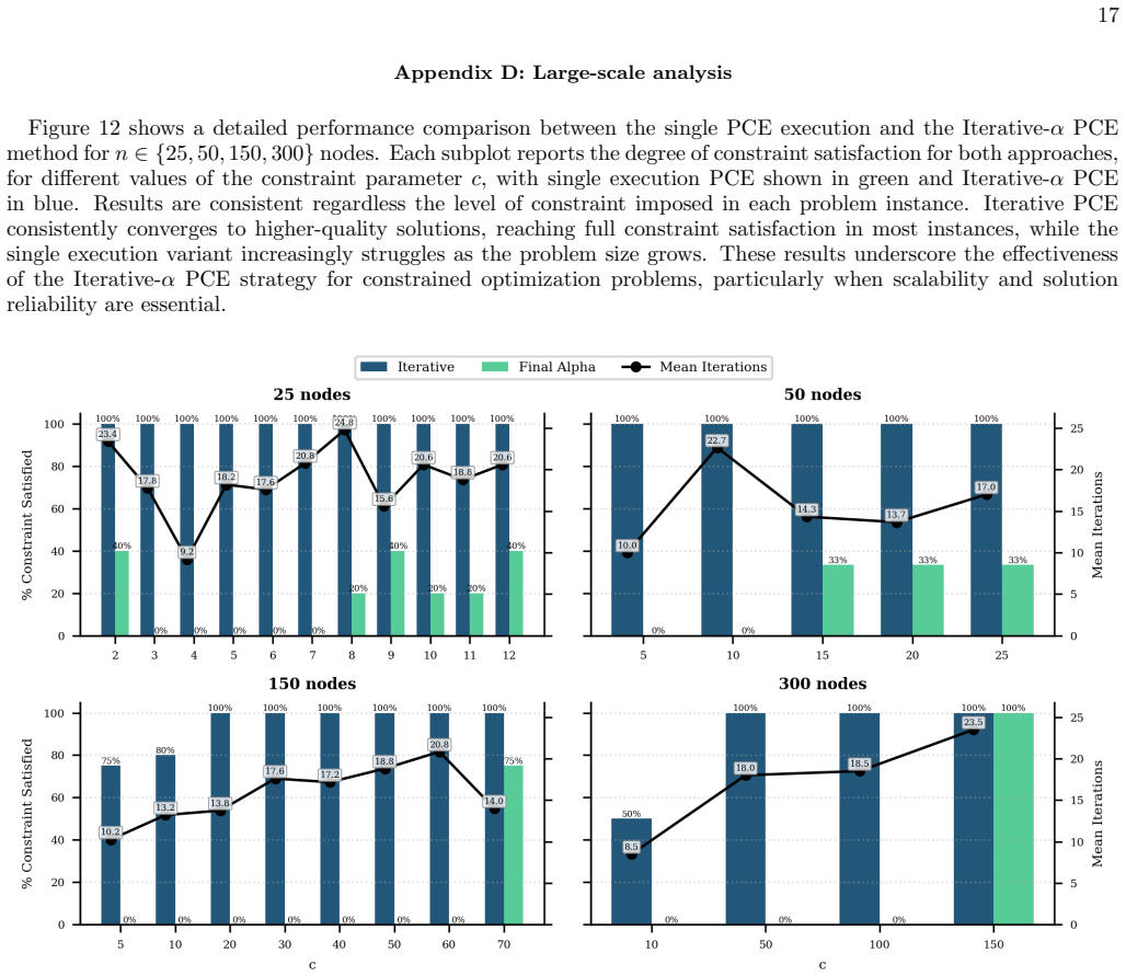
On its own terms, the central discovery is that binarization of the encoded variables is the gatekeeper for constraint satisfaction in PCE, and that the optimizer can be steered through binarization by a continuation on α. The constraint term in the relaxed loss can be lowered by fractional values of tanh(α⟨Π_i⟩) that do not correspond to any valid binary assignment, so feasible solutions emerge only when variables are driven to ±1. Standard PCE does not do this reliably: its constraint-success rate falls from 53% at 6 nodes to 22% at 25 nodes. Iterative-αPCE reverses that trend, reaching 100% success and full binarization for graphs up to 50 nodes and 88–95% for 150- and 300-node instances

Load-bearing premise

The load-bearing premise is that a single-layer alternating-gate circuit on 9 qubits, with a fixed assignment of order-k Pauli strings to variables, can actually represent near-optimal cuts of 300-variable instances once the α-continuation is applied.

Editorial extensions

If this is right

Constrained QUBOs no longer require one qubit per variable; the paper reports 300-variable budget-constrained MinCut instances run on 9-qubit circuits.
Feasibility no longer hinges on a hand-tuned sharpness parameter; the continuation schedule automatically drives variables to the binary domain across instances.
The number of stages (10–20) is nearly independent of problem size, so the added overhead of the iterative scheme grows only slowly as instances scale.
The derived penalty β(c) removes a second poorly transferable hyperparameter, leaving mainly the threshold M and initial α to be set.
The control experiment implies the performance gain is intrinsic to the path of α, not to the final α value, so the method is not equivalent to simply picking a better fixed parameter.

Reading between the lines

Editorial extensions of the paper, not claims the author makes directly.

The plateau-freezing explanation suggests a general recipe: any continuous relaxation whose discrete limit costs vanishing gradients can be scheduled by an analogous continuation, so PB-PCE-style schedules may transfer to other quantum and classical relaxed optimizers.
The paper leaves the mapping from Pauli strings to variables fixed; rerunning the n=300 experiments with several random permutations of that mapping would show whether the reported 9-qubit scalability is robust or an artifact of the particular encoding.
The single-variable α update is conservative; updating all variables below the threshold in one step could reduce the 10–20 stages while preserving the freezing mechanism, a modification that is directly testable.
The β(c) heuristic follows from an upper bound on the cut term for undirected weighted graphs; extending the derivation to directed or capacitated graphs would clarify how far the heuristic generalizes.

Share X Bluesky LinkedIn Reddit HN

Editorial analysis

A structured set of objections, weighed in public.

Desk editor's note, referee report, and a circularity audit.

Desk Editor's Note

read the letter

Here's the short version: I think this paper deserves referee time, but the flagship claim should be read as provisional. The Iterative-αPCE idea is simple and sensible—start with small α, increase gradually, warm-start from the previous solution. Continuation methods are standard in classical optimization, but this is the first application to PCE, and the paper earns that. The paired control (Iterative-α vs standard PCE at the same final α from the same run) is exactly the right experiment, and the result is clear: the iterative path, not just the final α, is responsible for the higher constraint-satisfaction rate. That is a genuine finding. The β(c) penalty bound in Appendix A is derived from an upper bound on cut value rather than fitted to data, which is more than one usually gets for penalty hyperparameters.

Soft spots are mostly concentrated in the large-scale section. The α-update changes from Algorithm 1 to Eq. (21) for n=150/300; M and α0 are retuned (Table XI), including a change in Pauli order k from 2 to 4. So the headline '300 variables with 9 qubits' is not produced by the algorithm validated on the small graphs. No error bars or run counts are reported for large graphs, and no code or data are shipped. The matched-pair cut-size comparison is also mildly biased in favor of Iterative-α: by conditioning on cases where both methods satisfy the constraint, you drop runs where standard PCE got lucky or where Iterative struggled, and at n=300 the cut-size advantage shrinks to 0.75%, which is within noise. The expressibility concern raised in the stress-test is real: the paper never checks whether the single-layer brickwork ansatz with the chosen Pauli strings can represent near-optimal feasible cuts at all. A control experiment asking the same ansatz to fit an SA-optimal bitstring would answer that cheaply, and its absence leaves the 300-node result more fragile than the small-instance results. This is not a fatal flaw in the central continuation idea—on n≤50 the evidence is solid—but it is a load-bearing gap for the scalability claim.

Minor: the title says Progressive-Binarization PCE while the text says Iterative-αPCE; that looks like an editorial inconsistency, not a substantive problem.

Who this is for: people working on PCE or few-qubit encodings for QUBO. They should read Sections IV and V. Send it to peer review with a request for code/data, a fixed-α warm-start comparison, an expressibility control, and run counts with error bars. I would cite the β(c) bound and the paired-control methodology, not the 300-node result, until it is independently verified.

Referee Report

4 major / 5 minor

Summary. The paper extends Pauli Correlation Encoding (PCE) to constrained combinatorial optimization, using budget-constrained MinCut as the test problem. In PCE, binary variables are encoded in the signs of expectation values of k-local Pauli strings on m qubits with m much smaller than the number of variables n. The authors show that standard fixed-α PCE has poor constraint satisfaction because tanh-binarization is incomplete, and that both α and β are hard to tune. They introduce Iterative-αPCE: start from a small α, optimize the circuit, identify the least-binarized variable, increase α so that this variable crosses a threshold M, and warm-start the next optimization from the previous parameters. On graphs of 6–25 nodes they report 100% constraint satisfaction and full binarization, and lower cut sizes than standard PCE run at the same final α. For 50–300 nodes, using a modified α-update and the QARP framework, they report 88–100% constraint success, with 300-node instances solved using 9-qubit circuits. They also derive a graph-degree-based upper bound for the penalty parameter β_c.

Significance. The core idea is sensible and the paired control—Iterative-α versus standard PCE at the same final α—is a good experimental design: it gives direct evidence that the continuation path, not merely the final α value, is responsible for the improvement. The derivation of β_c from an upper bound on the cut value (Appendix A) is explicit and not fitted to data. If the statistical and representational gaps identified below are closed, the method would be a genuinely useful few-qubit technique for constrained optimization. However, the flagship large-scale claim currently rests on unstated run counts, absent error bars, retuned hyperparameters, a modified update rule, and an unexamined expressibility assumption about the shallow fixed-Pauli-string ansatz. The paper is therefore promising but not yet fully supported.

major comments (4)

[V.A, Eq. (21); Table XI] The large-scale results are not produced by the algorithm validated in Tables III–V. Algorithm 1 line 7 updates α with α←α·arctanh(M)/arctanh(|tanh(α⟨Π_i⋆⟩)|), while Eq. (21) drops the arctanh in the denominator. In addition, Table XI changes k (2→3→4), M (0.90→0.95), and α0 (3→1) for the larger graphs. Claims about scaling to 150–300 nodes should therefore be stated as properties of this modified variant, not of Iterative-αPCE as characterized earlier. Please validate Eq. (21) on the small instances with the same paired control, or explicitly justify and separately benchmark the variant.
[V.B; Tables VII–IX] No number of runs, error bars, or confidence intervals are reported for n=50,150,300. The headline '88–100% constraint satisfaction' is uninterpretable without N: 88% could be 7/8 or 88/100. Similarly, the -0.75% CutSize difference at n=300 (Table VIII) is likely within noise. The paper should report N for every entry and give distributions or bootstrap confidence intervals for ε_c and CutSize, especially because the large-scale section is the basis of the abstract's central claim.
[V.B; Table X] The 300-variable/9-qubit result rests on an unverified representational assumption: a single-layer Brickwork ansatz with fixed order-k Pauli strings must be able to produce 300 expectation-value sign patterns that correspond to near-optimal feasible cuts. No expressibility analysis, no check that the ansatz can fit simulated-annealing-optimal bitstrings, and no comparison with a classical low-dimensional feature map are provided. Because k, M, and α0 change across sizes, the large-graph numbers may reflect instance structure rather than a general few-qubit encoding capability. Add a representability control and test on a broader family of random graphs before claiming that 300-variable instances are solved by 9 qubits.
[III.B; Table XI] The paper repeatedly states that Iterative-αPCE 'does not require any prior estimation of the parameter α,' but the method still depends on the threshold M and the initial α0, and Table XI shows that both were re-tuned for n=150/300. This weakens the transferability claim. Please provide a sensitivity analysis over M and α0, or state clearly that these are user-set hyperparameters with instance-dependent choices.

minor comments (5)

[Eqs. (4), (12)] Equation (4) includes L_reg, but Eq. (12), called the final expression, omits it. The relationship between the two expressions should be clarified.
[Notation throughout] The paper switches between x_i∈{0,1} and z_i∈{−1,1} and uses n for both the number of nodes and (in the α∼n^{k/2} discussion) the number of qubits. This makes Section IV.A and the regularization definition hard to follow.
[Typos and wording] Several typos and grammatical errors should be fixed: 'divissions', 'effectly', 'strenth', 'a' in the text around Eq. (21), and the Appendix D caption says n∈{18,50,150,300} while the text says n∈{25,50,150,300}.
[Reproducibility] No code or data availability statement is included, and the large-scale experiments use the proprietary QARP framework. The runtime comparison in Appendix E is helpful, but the absence of an open implementation limits reproducibility of the central numerical claims.
[References] Reference [10] is an incomplete citation to a Physical Review Research article and should include authors and year; reference [19] is likewise incomplete.

Circularity Check

1 steps flagged · score 2.0 of 10

Minor local circularity: the binarization metric shares its threshold with the algorithm's stopping rule; central constraint/cut results are not circular.

self definitional [Section IV (Binarization metric, Eq. 14); Section V Algorithm 1; Appendix C Table XI]
"2. Binarization: ... We consider that a variable tanh(α⟨Π_i⟩) is binarized if |tanh(α⟨Π_i⟩)|>0.9. ... Binarization = |V|/n ... Algorithm 1: 'until |tanh(α⟨Π_i⟩)| ≥ M ∀i' ... Appendix C Table XI: 'Threshold (M) 0.90'"

The binarization metric's threshold (>0.9) is the same numerical value as the algorithm's stopping threshold M, set to 0.90 in Table XI for every instance. Algorithm 1 terminates only when every variable satisfies |tanh(α⟨Π_i⟩)| ≥ M, so the paper's headline that Iterative-αPCE achieves 'full binarization' (Bin=1.00 in Tables V and IX) is substantially built into the stopping rule rather than independently measured. This is a local self-definitional alignment. It does not make the constraint-success or CutSize comparisons circular: those compare the iterative schedule against standard PCE at the same final α and against simulated-annealing baselines, and the β_c penalty is derived from an upper bound (Appendix A), not fitted.

full rationale

The central derivation chain is not circular. The penalty parameter β_c is obtained from a mathematical upper bound on the cut value in Appendix A, not from fitting to the reported results. The Iterative-αPCE is benchmarked against standard PCE at the matched final α value and against simulated annealing as an external baseline; no fitted parameter is renamed as a prediction. The self-citation to the authors' portfolio-optimization paper [8] appears only as background and is not load-bearing; the PCE method itself rests on the external work [7]. The skeptic's expressibility concern about the single-layer Brickwork ansatz and Pauli-string assignment is a real correctness/evidence gap, but it is not a circularity: the paper does not claim to derive expressibility from its own assumptions. The only localized circular element is that 'full binarization' is measured with the same 0.9 threshold that the continuation loop is designed to enforce, so that particular metric is partly tautological. Constraint satisfaction (88–100%) and cut-size quality remain non-tautological, independently benchmarked claims. Overall, no load-bearing circularity is present; the score reflects the minor self-definitional metric alignment.

Assumptions & free parameters 3 free parameters · 3 assumptions · 0 invented entities

The method introduces no new physical entities. It relies on the expressibility of a shallow parameterized circuit (domain assumption), the validity of noiseless simulation, and the tanh relaxation. Two hyperparameters (M, α0) are hand-set and re-tuned for larger instances; the large-scale α update formula (Eq. 21) is an ad hoc modification.

free parameters (3)

Binarization threshold M = 0.90 for n≤50; 0.95 for n≥150
Hand-set threshold in Algorithm 1; changed for larger graphs, indicating it does not transfer across instance sizes.
Initial α0 = 3 for n≤50; 1 for n≥150
Starting value of the tanh slope; changed for large instances because α0=3 prevented convergence.
Large-scale α update formula = α·arctanh(M)/|tanh(α⟨Π_i*⟩)|
Modified update (Eq. 21) used for n≥150; not derived, and differs from Algorithm 1's formula.

assumptions (3)

domain assumption A single-layer Brickwork ansatz with m qubits has sufficient expressibility to encode near-optimal solutions to budget-constrained MinCut instances with n≫m variables via Pauli-correlation expectation values.
Assumed throughout Sections IV–V; the paper does not analyze the expressibility or the fidelity of the encoding.
domain assumption Simulations in a noiseless statevector model are representative of the behavior claimed for the NISQ era.
All experiments use Qiskit/Qulacs simulators; no hardware or noise model is used, though the conclusions address NISQ suitability.
domain assumption The tanh relaxation preserves the global ordering of solutions so that minimizing the continuous loss yields a good bitstring after discretization.
Used to define the loss (Eq. 12); the paper's own Section IV shows this fails without iterative binarization, so the assumption is only valid under the proposed schedule.

how reviews work

0 comments

Cite this review

Pith. "Pith review of Progressive Binarization - Pauli Correlation Encoding: a Continuation Method for Constrained Optimization." pith.science (2026). https://pith.science/paper/SLAUZ4TA

@misc{pith2026260217479,
  author       = {Pith},
  title        = {Pith review of: Progressive Binarization - Pauli Correlation Encoding: a Continuation Method for Constrained Optimization},
  year         = {2026},
  howpublished = {\url{https://pith.science/paper/SLAUZ4TA}},
  note         = {Machine review of arXiv:2602.17479}
}

read the original abstract

Pauli Correlation Encoding (PCE) reduces the qubit requirements of quantum optimization by embedding the problem variables into the expectation values of Pauli observables, so that the number of qubits can be much smaller than the number of variables. PCE has not yet been studied for constrained optimization. We extend it to constrained combinatorial problems, using the budget-constrained MinCut as a case study, and show that the standard formulation fails to reliably enforce the constraint: feasibility hinges on the binarization of the encoded variables, which depends sensitively on hyperparameters that are hard to tune and do not transfer across instances. To address this, we introduce Progressive-Binarization PCE (PB-PCE), an adaptive continuation scheme that progressively increases the binarization parameter while re-optimizing the circuit from the previous solution, driving the variables towards the binary domain. PB-PCE attains near-complete constraint satisfaction (88--100\%) and smaller cut sizes than standard PCE, with a number of stages (10--20) essentially independent of problem size, solving instances of up to 300 variables with only 9-qubit circuits.

Figures

Figures reproduced from arXiv: 2602.17479 by the authors.

**Figure 2.** FIG. 2: (a) tanh ( [PITH_FULL_IMAGE:figures/full_fig_p004_2.png] view at source ↗

**Figure 3.** FIG. 3: (a) Constraint success ratio [PITH_FULL_IMAGE:figures/full_fig_p005_3.png] view at source ↗

Figures from the paper (9 more)

**Figure 4.** Figure 4: FIG. 4: (a) Constraint success ratio [PITH_FULL_IMAGE:figures/full_fig_p006_4.png]

**Figure 5.** Figure 5: FIG. 5: Constraint succeess ratio [PITH_FULL_IMAGE:figures/full_fig_p007_5.png]

**Figure 6.** Figure 6: FIG. 6: Example of a cut separating two nodes ( [PITH_FULL_IMAGE:figures/full_fig_p008_6.png]

**Figure 7.** Figure 7: FIG. 7: Constraint success ratio [PITH_FULL_IMAGE:figures/full_fig_p008_7.png]

**Figure 8.** Figure 8: FIG. 8: Effect of the regularization strength [PITH_FULL_IMAGE:figures/full_fig_p009_8.png]

**Figure 9.** Figure 9: shows the distribution of final values αf reached across all executions of the Iterative-α PCE. No clear concentration around a specific value of αf is observed. Instead, the distribution spans several orders of magnitude, ranging approximately from 102 to 104 , with …

**Figure 10.** Figure 10: FIG. 10: Evolution of constraint satisfaction and binarization during the Iterative- [PITH_FULL_IMAGE:figures/full_fig_p011_10.png]

**Figure 11.** Figure 11: FIG. 11: Evolution of the encoded variables during a single execution of the Iterative- [PITH_FULL_IMAGE:figures/full_fig_p016_11.png]

**Figure 12.** Figure 12: FIG. 12: Performance comparison between iterative- [PITH_FULL_IMAGE:figures/full_fig_p017_12.png]

Discussion (0). Continue with ORCID to comment.

Forward citations

Cited by 1 Pith paper

Reviewed papers in the Pith corpus that reference this work. Sorted by Pith novelty score. Full citation record

Scalable Variational Quantum Optimization via Pauli Correlation Encoding: Application to Large-Scale Power Demand Portfolio Optimization
quant-ph 2026-07 conditional novelty 5.0 of 10

Pauli correlation encoding solves dense power-demand portfolio QUBOs up to m=10,296 with ~14 qubits and normalized cost gaps ~10^{-4}, with behavior set by continuous-to-discrete correlator resolution.

Reference graph

Works this paper leans on

33 extracted references · 3 linked inside Pith · cited by 1 Pith paper

[1]

Prepare a parametrized quantum state|Ψ( ⃗θ)⟩
[2]

Compute the expectation values⟨Π i⟩to evaluate the loss functionL( ⃗θ)
[3]

Use a classical optimizer to update the parameters for the next iteration
[4]

Repeat the procedure until the loss is minimized
[5]

, xn) withx i = sign (⟨Πi⟩)

Once convergence is reached , construct the bit- string solution x= (x 1, x2, . . . , xn) withx i = sign (⟨Πi⟩)
[6]

1 2 nX i zi + 1 ! −c #2 = =β

Compute the cut size value using the bitstring so- lution in the original QUBO expression Eq. (5). III. BUDGET-CONSTRAINTED MINCUT PROBLEMS Many real-world optimization problems involve addi- tional constraints that go beyond the standard uncon- strained MinCut or MaxCut formulations. In particular, budget or balance constraints naturally arise in applica...
[7]

Sciorilli, L

M. Sciorilli, L. Borges, T. L. Patti, D. Garc ´ ıa-Mart ´ ın, G. Camilo, A. Anandkumar, and L. Aolita, Towards large-scale quantum optimization solvers with few qubits, Nature Communications16, 476 (2025), publisher: Na- ture Publishing Group UK London

2025
[8]

For each value ofc, the overall performance of PCE is primarily governed by the choice ofα

Show all 33 references

[9]

In practice, similar performance levels are observed forβ∼10 2,β∼10 3, andβ∼10 4

For fixed values ofαandc, there is no clear range ofβvalues that consistently yields optimal perfor- mance. In practice, similar performance levels are observed forβ∼10 2,β∼10 3, andβ∼10 4
[10]

For example, forα= 4 andc= 5, a peak in the constraint success ratioε c is observed atβ= 5000, whereas a slight increase toβ= 7000 causesε c to drop to zero

At fixedαandc, the performance is highly sensitive to the specific value ofβwithin the same order of magnitude. For example, forα= 4 andc= 5, a peak in the constraint success ratioε c is observed atβ= 5000, whereas a slight increase toβ= 7000 causesε c to drop to zero. Several...
[11]

This is evident from the highlighted bars in Figure 5, which indicate the highestε c for each configuration

The value ofβthat yields the best performance is not transferable across different (α, c) configu- rations. This is evident from the highlighted bars in Figure 5, which indicate the highestε c for each configuration. For instance, whileβ= 3000 and β= 70000 provide the best res...
[12]

This trend is observed across the full range ofβvalues and is also reflected in the results obtained usingβ c, whereε c increases from 0.50 at α= 4 to 0.92 atα= 16

The overall performance is predominantly deter- mined byα. This trend is observed across the full range ofβvalues and is also reflected in the results obtained usingβ c, whereε c increases from 0.50 at α= 4 to 0.92 atα= 16
[13]

The proposed penalty parameterβ c yields equal or improved performance using a single value for allc, independently ofα. In conclusion, the proposed expression forβ(c) yields consistent performance and can therefore be used to study the algorithm in a systematic manner, withou...

2000
[14]

Abbas, A

A. Abbas, A. Ambainis, B. Augustino, A. B¨ artschi, H. Buhrman, C. Coffrin, G. Cortiana, V. Dunjko, D. J. Egger, B. G. Elmegreen, and others, Challenges and op- portunities in quantum optimization, Nature Reviews Physics , 1 (2024), publisher: Nature Publishing Group

2024
[15]

Cerezo, A

M. Cerezo, A. Arrasmith, R. Babbush, S. C. Benjamin, S. Endo, K. Fujii, J. R. McClean, K. Mitarai, X. Yuan, L. Cincio, and others, Variational quantum algorithms, Nature Reviews Physics3, 625 (2021), publisher: Nature Publishing Group UK London

2021
[16]

Farhi, J

E. Farhi, J. Goldstone, and S. Gutmann, A quan- tum approximate optimization algorithm, arXiv preprint arXiv:1411.4028 (2014)

2014 arXiv
[17]

Peruzzo, J

A. Peruzzo, J. McClean, P. Shadbolt, M.-H. Yung, X.-Q. Zhou, P. J. Love, A. Aspuru-Guzik, and J. L. O’brien, A variational eigenvalue solver on a photonic quantum pro- cessor, Nature communications5, 4213 (2014), publisher: Nature Publishing Group UK London

2014
[18]

D. d. Falco and D. Tamascelli, An introduction to quan- tum annealing, RAIRO - Theoretical Informatics and Ap- 14 plications45, 99 (2011)

2011
[19]

Yarkoni, E

S. Yarkoni, E. Raponi, T. B¨ ack, and S. Schmitt, Quan- tum annealing for industry applications: introduction and review, Reports on Progress in Physics85, 104001 (2022), publisher: IOP Publishing

2022
[20]

Javadi-Abhari, M

A. Javadi-Abhari, M. Treinish, K. Krsulich, C. J. Wood, J. Lishman, J. Gacon, S. Martiel, P. D. Nation, L. S. Bishop, A. W. Cross, and others, Quantum computing with Qiskit, arXiv preprint arXiv:2405.08810 (2024). 15 Appendix A:β c calculous We introduce here the full mathemat...

2024 arXiv
[21]

V. P. Soloviev and M. Krompiec, Large-scale portfolio optimization using Pauli Correlation Encoding, arXiv preprint arXiv:2511.21305 (2025)

2025
[22]

Pauli Correlation Encoding to reduce Maxcut require- ments (), publication Title: IBM Quantum Documenta- tion
[23]

Variational quantum optimization with multibasis encod- ings|Phys. Rev. Research ()
[24]

Puerto and J

J. Puerto and J. L. Sainz-Pardo, Budget-constrained cut problems (2023), arXiv:2308.07063 [math]

2023 arXiv
[25]

Engelberg, J

R. Engelberg, J. K¨ onemann, S. Leonardi, and J. S. Naor, Cut problems in graphs with a budget constraint, Jour- nal of Discrete Algorithms 2004 Symposium on String Processing and Information Retrieval,5, 262 (2007)

2004
[26]

Chekuri and A

C. Chekuri and A. Kumar, Maximum Coverage Prob- lem with Group Budget Constraints and Applications, inApproximation, Randomization, and Combinatorial Optimization. Algorithms and Techniques, edited by K. Jansen, S. Khanna, J. D. P. Rolim, and D. Ron (Springer, Berlin, Heidelbe...

2004
[27]

Takei, W

R. Takei, W. Chen, Z. Clawson, S. Kirov, and A. Vladimirsky, Optimal Control with Budget Con- straints and Resets, SIAM Journal on Control and Opti- mization53, 712 (2015), publisher: Society for Industrial and Applied Mathematics

2015
[28]

Shi and B

W. Shi and B. Hong, Resource Allocation with a Bud- get Constraint for Computing Independent Tasks in the Cloud, in2010 IEEE Second International Conference on Cloud Computing Technology and Science(2010) pp. 327–334

2010
[29]

K. Rose, E. Gurewitz, and G. Fox, Constrained clustering as an optimization method, IEEE Transactions on Pat- tern Analysis and Machine Intelligence15, 785 (1993)

1993
[30]

P. J. Van Laarhoven and E. H. Aarts, Simulated an- nealing, inSimulated annealing: Theory and applications (Springer, 1987) pp. 7–15

1987
[31]

J. A. Nelder and R. Mead, A Simplex Method for Func- tion Minimization, The Computer Journal7, 308 (1965)

1965
[32]

Exact and sequential penalty weights in quadratic un- constrained binary optimisation with a digital annealer| Proceedings of the Genetic and Evolutionary Computa- tion Conference Companion ()
[100]

However, when evaluating the cut size, larger values ofαdo not systematically lead to improved solutions. In 6 0 250 500 750 1000 1250 1500 1750 2000 0.0 0.2 0.4 0.6 0.8 1.0 Constraint Success ( c) (a) 0.0 0.5 1.0 Binarization (b) 0 500 1000 1500 2000 0.0 1.0 2.0 3.0 4.0 CutSi...

2000

Pith tools

Reviewed August 2, 2026 · model on record in the stance chip above.

[1] [1]

Prepare a parametrized quantum state|Ψ( ⃗θ)⟩

[2] [2]

Compute the expectation values⟨Π i⟩to evaluate the loss functionL( ⃗θ)

[3] [3]

Use a classical optimizer to update the parameters for the next iteration

[4] [4]

Repeat the procedure until the loss is minimized

[5] [5]

, xn) withx i = sign (⟨Πi⟩)

Once convergence is reached , construct the bit- string solution x= (x 1, x2, . . . , xn) withx i = sign (⟨Πi⟩)

[6] [6]

1 2 nX i zi + 1 ! −c #2 = =β

Compute the cut size value using the bitstring so- lution in the original QUBO expression Eq. (5). III. BUDGET-CONSTRAINTED MINCUT PROBLEMS Many real-world optimization problems involve addi- tional constraints that go beyond the standard uncon- strained MinCut or MaxCut formulations. In particular, budget or balance constraints naturally arise in applica...

[7] [7]

Sciorilli, L

M. Sciorilli, L. Borges, T. L. Patti, D. Garc ´ ıa-Mart ´ ın, G. Camilo, A. Anandkumar, and L. Aolita, Towards large-scale quantum optimization solvers with few qubits, Nature Communications16, 476 (2025), publisher: Na- ture Publishing Group UK London

2025

[8] [8]

For each value ofc, the overall performance of PCE is primarily governed by the choice ofα