REVIEW 3 major objections 5 minor 84 references
Segmenting Low-Contrast XCTs of Concrete: An Unsupervised Approach
T0 review · 3 major / 5 minor · reviewed 2026-08-02 · deepseek-v4-flash
Pith's one-line read This paper shows that a U-Net trained with self-annotated superpixel labels can separate aggregate from mortar in low-contrast concrete XCT images, outperforming direct greyscale thresholding on out-of-distribution data.
desk verdict Useful, honest adaptation of Kanezaki-style self-annotation to low-contrast concrete XCT, but the headline claim against direct thresholding is not yet controlled because of manual per-image thresholds and asymmetric postprocessing. read the letter →
The pith
A machine-rendered reading of the paper's core claim, the machinery that carries it, and where it could break.
The reading
What carries the argument
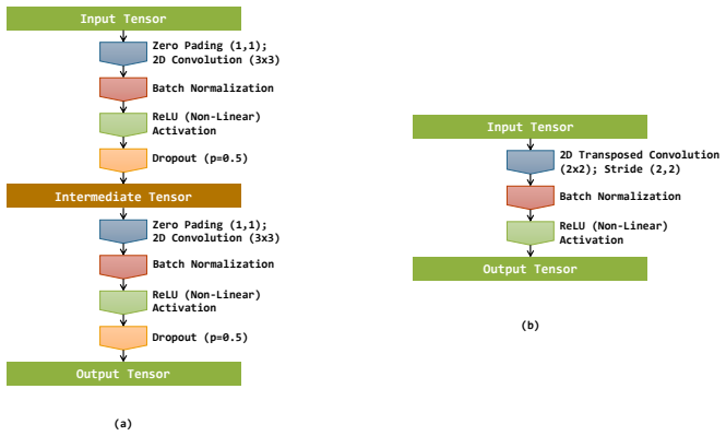
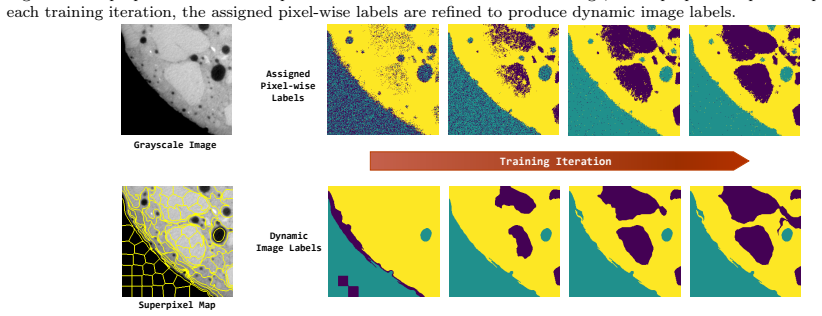
The engine is the superpixel-refinement self-annotation loop. SLIC partitions each image into small contiguous regions of perceptual similarity; the most frequent predicted class in each region becomes the label for all its pixels, producing dynamic image labels that are fed back as training targets. This converts noisy, pixel-level CNN outputs into spatially coherent pseudo-labels and ties local superpixel structure to the global context captured by the network's receptive field. Per-channel normalization of the output prevents the model from collapsing to a single phase, although the paper notes it remains fragile under class imbalance. The architecture is a U-Net-style encoder-decoder wit
What would settle it
Compare the superpixel-refined training labels against the 16 manually annotated slices: if superpixels frequently straddle aggregate-mortar boundaries in low-contrast regions and the model's errors correlate with those straddles, the refinement assumption fails. More directly, train the same pipeline with deliberately misaligned superpixels (e.g., extreme compactness or oversized superpixels); if aggregate identification accuracy does not degrade, the superpixel-alignment assumption is not load-bearing.
Extended reading notes
Core claim
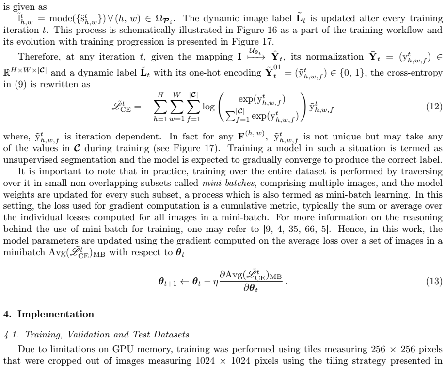
The paper's central claim is that a convolutional encoder-decoder network can learn to separate aggregate from mortar in low-contrast concrete XCT images using no labelled data for those phases, and that the resulting aggregate segmentations are more accurate than direct greyscale thresholding. The self-annotation loop works as follows: after each training pass, per-pixel predictions are normalized per output channel, converted to hard labels by argmax, and then refined by replacing every pixel's label with the majority label of its SLIC superpixel. These refined labels—called dynamic image labels—are used as the cross-entropy training targets for the next iteration, evolving as the model im
Load-bearing premise
The load-bearing premise is that SLIC superpixels stay inside single phases and that the majority predicted class within a superpixel is the true phase; in low-contrast regions where superpixels straddle aggregate-mortar boundaries, wrong labels are fed back into training and the model can learn to reproduce those errors.
Editorial extensions
If this is right
- Concrete XCT scans can be segmented into aggregate and mortar phases without manual annotation, removing the main bottleneck to using XCT in concrete mechanics.
- Thresholding the aggregate-specific channel of the normalized network output identifies aggregates better than thresholding raw XCT slices, so the network acts as an intensity transform that sharpens phase separability.
- A purely unsupervised three-phase setup fails to isolate porosity; the semi-supervised variant, which thresholds only the easily separable pore phase, gives unambiguous three-phase labels.
- The learned segmentation can bootstrap supervised training: the paper explicitly proposes using its outputs as initial labels for fine-tuning on new concrete datasets.
- The method inherits concrete failure modes: aggregates near the sample periphery are missed and closely spaced small aggregates are merged, so downstream users should expect those behaviors.
Reading between the lines
- A natural testable extension is to apply the same self-annotation loop to other low-contrast multiphase materials with a known phase count and check whether the superpixel-mode assumption degrades as phase-boundary contrast drops.
- The reported periphery failure may be a receptive-field or padding artifact rather than a fundamental limit; training on full slices or using border-aware crops could recover those aggregates.
- Because the paper flags per-channel normalization as fragile under class imbalance, a class-balanced or entropy-regularized alternative could make the fully unsupervised three-phase case succeed and remove the need to threshold porosity.
- The dynamic-label loop is a form of self-training, so its convergence likely depends on initial random predictions being slightly better than chance within each superpixel; this could be tested by seeding training with a simple intensity prior.
Signed reviews
Editorial analysis
A structured set of objections, weighed in public.
Referee Report
Summary. The paper presents a self-annotation-based segmentation pipeline for low-contrast X-ray CT images of concrete, targeting three phases: aggregate, mortar, and porosity. A U-Net is trained without manually labeled aggregate/mortar data; per-pixel predictions are converted into 'dynamic image labels' by per-channel normalization, argmax classification, and SLIC superpixel refinement (Eq. 12, Section 3.4). Three training configurations are tested: fully unsupervised with 3 channels (US3), fully unsupervised with 4 channels (US4), and semi-supervised with 3 channels where porosity labels are provided by thresholding (SS3). On a held-out XCT sample with 16 manually annotated slices, the authors compare aggregate segmentation obtained by thresholding the aggregate-specific logit channel of SS3 against direct grayscale thresholding of the original XCT images, reporting that the proposed method consistently outperforms direct thresholding across IoU, precision, sensitivity, and F1. The authors also document limitations, including failure of the fully unsupervised variants to resolve porosity and systematic errors near sample peripheries and between closely spaced aggregates.
Significance. If the empirical claim is substantiated, the work has practical value: it offers a way to train a segmentation model for concrete XCT without manually annotated aggregate/mortar labels, which is a real bottleneck for morphology-based analysis in experimental mechanics. The paper also ships processed data, code, and model weights via Zenodo, which supports reproducibility and follow-up work. The held-out manual ground truth provides a meaningful independent check on the self-annotation loop. However, the headline claim is currently under-supported because the comparison against direct thresholding is not controlled, and the only fully successful configuration (SS3) is semi-supervised rather than unsupervised. The contribution of the self-annotation mechanism itself, as distinct from per-image threshold tuning and heavier morphological postprocessing, is not yet isolated.
major comments (3)
- [§7.2, Fig. 31; §6; §5.3] The central claim that logit thresholding of the SS3 output 'consistently outperformed' direct grayscale thresholding is confounded. Section 6 states that the threshold applied to the aggregate channel is 'unique' for each image but gives no selection rule, and Section 5.3 explicitly omits thresholding details. Direct thresholding also appears to be manually tuned. Furthermore, the postprocessing chains differ: the logit pipeline applies hole filling to 512 px, binary erosion, removal of objects <128 px, and final dilation, while the direct-threshold baseline only removes objects <128 px and holes <256 px. Reported gains could therefore arise from per-image threshold selection and extra morphological operations rather than from the learned aggregate/mortar separation. Please fix both operations to a reproducible rule (e.g., Otsu or a fixed percentile on each channel) and use identical po
- [§5.1–§5.3; Abstract] The paper is framed as an 'unsupervised approach,' but the fully unsupervised variants US3 and US4 both fail to unambiguously segment the porous phase (Figs. 21–24). The successful SS3 configuration uses thresholded porosity labels during training, making it semi-supervised. The abstract's claim that the methodology consistently outperforms direct thresholding refers to SS3, not to the unsupervised variants. This is a load-bearing mismatch between the title/abstract and the experimental results. Either temper the 'unsupervised' claims to 'semi-supervised for porosity, unsupervised for aggregate/mortar,' or demonstrate a fully unsupervised configuration that resolves all three phases.
- [§3.4, Eq. (12)] The self-annotation mechanism rests on the assumption that the most frequent predicted class within a SLIC superpixel is the correct semantic label for all pixels in that superpixel. If superpixels cross aggregate/mortar boundaries—which is likely in low-contrast regions—incorrect labels are fed back as training targets. The assumption is stated but never validated, e.g., by comparing superpixel boundaries against the manually annotated test slices or by measuring boundary recall/precision. A quantitative sanity check on the 16 annotated slices, or a sensitivity analysis over SLIC compactness and superpixel count, would materially strengthen the claim that the self-annotation loop is learning meaningful phase boundaries rather than propagating its own errors.
minor comments (5)
- [§2.1] Typo: 'numcerical' should be 'numerical.' Also, the description of beam-hardening correction would benefit from a reference or more detail on how the manual parameter choice affects downstream slices.
- [§5, Fig. 20] The loss curves are averaged over 10 training runs, but the qualitative results are shown for a single unspecified run. Please state clearly whether the presented segmentation examples are representative of all runs and whether the quantitative evaluation in Fig. 31 uses one model or an ensemble/average.
- [§7.2] Only aggregate-phase metrics are reported. While mortar is complementary to aggregate, porosity is not evaluated quantitatively. Since porosity is a key phase in concrete morphology and SS3 is the only configuration that resolves it, reporting porosity IoU on the same ground truth would make the evaluation more complete.
- [Eq. (10)] The normalization in Eq. (10) uses the per-image mean and variance of each channel, but the notation does not make clear whether these statistics are computed per tile, per image, or per batch. Please clarify, as this affects the interpretation of the 'dynamic labels' in minibatch training.
- [§6] The suggestion to interpolate thresholds across slices using PCHIP is useful, but the manuscript does not state how many slices are needed for reliable interpolation or how sensitive the final metrics are to the choice of interpolation points. A short experiment or guidance would improve practical reproducibility.
Circularity Check
No significant circularity: the central empirical claim is grounded in held-out manual annotations, and the self-annotation loop is an explicit training mechanism, not a disguised restatement of the result.
full rationale
The self-annotation procedure (Eqs. 10-12) does define training targets as a function of the model's own normalized predictions (argmax followed by superpixel mode), so in isolation the training objective is self-referential. However, the paper's central claim is not that these dynamic labels are correct by construction; it is that a U-Net trained with this objective generalizes to a held-out XCT sample (TPR) and, after postprocessing, matches manually annotated ground truth better than direct greyscale thresholding. That evaluation uses external manual annotations, so the comparison does not reduce to the model's own labels. The postprocessing threshold is described as 'unique' per image with no selection rule, and the morphological postprocessing differs between the proposed and baseline pipelines; this is a reproducibility/confounding concern about the empirical comparison, not a definitional circularity. No load-bearing self-citations or imported uniqueness/ansatz claims were found. The weaknesses acknowledged in Section 8 (porosity ambiguity, periphery aggregates, small-aggregate clumping, per-channel normalization) are honest limitations rather than circular reasoning.
Assumptions & free parameters
free parameters (5)
- SLIC compactness
- Number of superpixels
- Threshold for halo removal
- Threshold for aggregate channel binarization
- Morphological postprocessing parameters =
fill holes ≤512px, remove objects <128px, final dilation, remove <256px
assumptions (4)
- domain assumption SLIC superpixels correspond to perceptually similar regions that align with phase boundaries
- ad hoc to paper The most frequent class within a superpixel is the correct semantic label for all pixels in it
- domain assumption Concrete can be segmented into three phases: aggregate, mortar, and porosity
- domain assumption The receptive field of the U-Net is sufficient to capture global context for each pixel
Cite this review
Pith. "Pith review of Segmenting Low-Contrast XCTs of Concrete: An Unsupervised Approach." pith.science (2026). https://pith.science/paper/HSALGSXG
@misc{pith2026260300127,
  author       = {Pith},
  title        = {Pith review of: Segmenting Low-Contrast XCTs of Concrete: An Unsupervised Approach},
  year         = {2026},
  howpublished = {\url{https://pith.science/paper/HSALGSXG}},
  note         = {Machine review of arXiv:2603.00127}
}
read the original abstract
X-Ray Computed Tomography (XCT) is a compelling tool in experimental mechanics, capable of non-destructively extracting information pertaining to the internal morphology of materials. For materials with random heterogeneous morphology such as concrete, such information is of particular relevance since it allows for studies of morphology-related behaviour and for predictive modelling. Nevertheless, XCT images require semantic segmentation for practical usage. Here, concrete poses a unique challenge due to the similar X-ray attenuation coefficients of aggregates and mortar, which result in low contrast between the two phases in the ensuing XCT images. As such, purely intensity-dependent semantic segmentation tools remain unfeasible. While vision transformers (ViTs) and convolutional neural networks (CNNs) are proven techniques for semantic segmentation in such challenging cases, they typically require labelled training data, which is often unavailable for concrete or resource-intensive to obtain, thereby limiting their relevance. To address this challenge, a self-annotation technique is presented here that leverages superpixel algorithms to identify perceptually similar local regions in an image and relates them to the global context by utilizing the receptive field of a CNN-based model. This enables the model to learn a global-local relationship in the images and facilitates the identification of semantically similar structures. When evaluated against manually annotated ground truth on out-of-distribution data, the proposed methodology consistently outperformed direct greyscale thresholding across all pertinent metrics, demonstrating improved discernibility between aggregates and mortar, and providing the most favourable balance of sensitivity and precision for aggregate-phase identification.
Figures


Figures from the paper (28 more)






Reference graph
Works this paper leans on
-
[1]
Achanta, R., Shaji, A., Smith, K., Lucchi, A., Fua, P., and Süsstrunk, S. (2010). Slic superpixels
2010
-
[2]
Bajcsy, P., Feldman, S., Majurski, M., Snyder, K., and Brady, M. (2020). Approaches to training multiclass semantic image segmentation of damage in concrete.Journal of Microscopy, 279(2):98–113
2020
-
[3]
S., Wang, C., Zhou, X., and Hassan, M
Bangaru, S. S., Wang, C., Zhou, X., and Hassan, M. (2022). Scanning electron microscopy (sem) image segmentation for microstructure analysis of concrete using u-net convolutional neural network. Automation in Construction, 144:104602
2022
-
[4]
Bengio, Y. (2012). Practical recommendations for gradient-based training of deep architectures. In Neural networks: Tricks of the trade: Second edition, pages 437–478. Springer
2012
-
[5]
Bishop, C. M. and Bishop, H. (2023).Deep learning: Foundations and concepts. Springer Nature
2023
-
[6]
and van Mier, J
Bisschop, J. and van Mier, J. G. (2008). Effect of aggregates and microcracks on the drying rate of cementitious composites.Cement and Concrete Research, 38(10):1190–1196
2008
-
[7]
Böhm, R., Stiller, J., Behnisch, T., Zscheyge, M., Protz, R., Radloff, S., Gude, M., and Hufenbach, W. (2015). A quantitative comparison of the capabilities of in situ computed tomography and conventional computed tomography for damage analysis of composites.Composites Science and Technology, 110:62– 68
2015
-
[8]
C., Apley, D
Bostanabad, R., Zhang, Y., Li, X., Kearney, T., Brinson, L. C., Apley, D. W., Liu, W. K., and Chen, W. (2018). Computational microstructure characterization and reconstruction: Review of the state-of-the-art techniques.Progress in Materials Science, 95:1–41
2018
Show all 84 references
-
[9]
Bottou, L. (2012). Stochastic gradient descent tricks. InNeural networks: tricks of the trade: second edition, pages 421–436. Springer
2012
-
[10]
Brisard, S., Serdar, M., and Monteiro, P. J. (2020). Multiscale x-ray tomography of cementitious materials: A review.Cement and Concrete Research, 128:105824
2020
-
[11]
P., Lunardelli, M., Leusmann, T., Varady, P
Carrara, P., Kruse, R., Bentz, D. P., Lunardelli, M., Leusmann, T., Varady, P. A., and De Lorenzis, L. (2018). Improved mesoscale segmentation of concrete from 3d x-ray images using contrast enhancers. Cement and Concrete Composites, 93:30–42
2018
-
[12]
Chen, B., Zhang, H., Wang, G., Huo, J., Li, Y., and Li, L. (2023). Automatic concrete infrastructure crack semantic segmentation using deep learning.Automation in Construction, 152:104950
2023
-
[13]
Chen, L., Shan, W., and Liu, P. (2021). Identification of concrete aggregates using k-means clustering and level set method. InStructures, volume 34, pages 2069–2076. Elsevier
2021
-
[14]
Cheng, B., Schwing, A., and Kirillov, A. (2021). Per-pixel classification is not all you need for semantic segmentation.Advances in neural information processing systems, 34:17864–17875
2021
-
[15]
Coenen, M., Schack, T., Beyer, D., Heipke, C., and Haist, M. (2021). Semi-supervised segmenta- tion of concrete aggregate using consensus regularisation and prior guidance.ISPRS Annals of the Photogrammetry, Remote Sensing and Spatial Information Sciences V-2-2021 (2021), 2:83–91
2021
-
[16]
L., Nardelli, M
Curtarolo, S., Hart, G. L., Nardelli, M. B., Mingo, N., Sanvito, S., and Levy, O. (2013). The high-throughput highway to computational materials design.Nature materials, 12(3):191–201
2013
-
[17]
Dong, Y., Su, C., Qiao, P., and Sun, L. (2020). Microstructural crack segmentation of three- dimensional concrete images based on deep convolutional neural networks.Construction and Building Materials, 253:119185
2020
-
[18]
Fritsch, F. N. and Butland, J. (1984). A method for constructing local monotone piecewise cubic interpolants.SIAM journal on scientific and statistical computing, 5(2):300–304. 28
1984
-
[19]
Fujiwara, T. (2008). Effect of aggregate on drying shrinkage of concrete.Journal of Advanced Concrete Technology, 6(1):31–44
2008
-
[20]
T., Niezgoda, S
Fullwood, D. T., Niezgoda, S. R., Adams, B. L., and Kalidindi, S. R. (2010). Microstructure sensitive design for performance optimization.Progress in Materials Science, 55(6):477–562
2010
-
[21]
and Bengio, Y
Glorot, X. and Bengio, Y. (2010). Understanding the difficulty of training deep feedforward neu- ral networks. InProceedings of the thirteenth international conference on artificial intelligence and statistics, pages 249–256. JMLR Workshop and Conference Proceedings
2010
-
[22]
Gonzalez, R. C. (2009).Digital image processing. Pearson education india
2009
-
[23]
(2016).Deep Learning
Goodfellow, I., Bengio, Y., and Courville, A. (2016).Deep Learning. MIT Press.http://www. deeplearningbook.org
2016
-
[24]
and Jirásek, M
Havlásek, P. and Jirásek, M. (2016). Multiscale modeling of drying shrinkage and creep of concrete. Cement and concrete research, 85:55–74
2016
-
[25]
Havlásek, P., Šmilauer, V., Dohnalová, L., and Sovják, R. (2021). Shrinkage-induced deformations and creep of structural concrete: 1-year measurements and numerical prediction.Cement and Concrete Research, 144:106402
2021
-
[26]
He, K., Gkioxari, G., Dollár, P., and Girshick, R. (2017). Mask r-cnn. InProceedings of the IEEE international conference on computer vision, pages 2961–2969
2017
-
[27]
Hilloulin, B., Bekrine, I., Schmitt, E., and Loukili, A. (2022). Modular deep learning segmentation algorithm for concrete microscopic images.Construction and Building Materials, 349:128736
2022
-
[28]
Hufenbach, W., Böhm, R., Gude, M., Berthel, M., Hornig, A., Ručevskis, S., and Andrich, M. (2012). A test device for damage characterisation of composites based on in situ computed tomography. Composites Science and Technology, 72(12):1361–1367
2012
-
[29]
Idiart, A., Bisschop, J., Caballero, A., and Lura, P. (2012). A numerical and experimental study of aggregate-induced shrinkage cracking in cementitious composites.Cement and Concrete Research, 42(2):272–281
2012
-
[30]
Batchnormalization: Acceleratingdeepnetworktrainingbyreducing internal covariate shift
Ioffe, S.andSzegedy, C.(2015). Batchnormalization: Acceleratingdeepnetworktrainingbyreducing internal covariate shift. InInternational conference on machine learning, pages 448–456. pmlr
2015
-
[31]
Jung, C., Müsebeck, F., Barisin, T., Schladitz, K., Redenbach, C., Kiesche, M., and Pahn, M. (2022). Towards automatic crack segmentation in 3d concrete images. In11th conf. ind. comput. tomogr.(ICT)
2022
-
[32]
R., Buzzy, M., Boyce, B
Kalidindi, S. R., Buzzy, M., Boyce, B. L., and Dingreville, R. (2022). Digital twins for materials. Frontiers in Materials, 9:818535
2022
-
[33]
F., Simpson, J
Kamnitsas, K., Ledig, C., Newcombe, V. F., Simpson, J. P., Kane, A. D., Menon, D. K., Rueckert, D., and Glocker, B. (2017). Efficient multi-scale 3d cnn with fully connected crf for accurate brain lesion segmentation.Medical image analysis, 36:61–78
2017
-
[34]
Kanezaki, A. (2018). Unsupervised image segmentation by backpropagation. In2018 IEEE inter- national conference on acoustics, speech and signal processing (ICASSP), pages 1543–1547. IEEE
2018
-
[35]
S., Mudigere, D., Nocedal, J., Smelyanskiy, M., and Tang, P
Keskar, N. S., Mudigere, D., Nocedal, J., Smelyanskiy, M., and Tang, P. T. P. (2016). On large-batch training for deep learning: Generalization gap and sharp minima.arXiv preprint arXiv:1609.04836
2016 arXiv
-
[36]
H., Park, K., et al
Kim, H.-T., Han, T.-S., Lee, Y. H., Park, K., et al. (2024). Recursive aggregate segmentation by erosion and reconstitution (raser) to characterize concrete microstructure using complementarity of x-ray and neutron computed tomography.Cement and Concrete Composites, 148:105437. 29
2024
-
[37]
A., Park, K., et al
Kim, H.-T., Szilágyi, V., Kis, Z., Szentmiklósi, L., Glinicki, M. A., Park, K., et al. (2021). Recon- struction of concrete microstructure using complementarity of x-ray and neutron tomography.Cement and Concrete Research, 148:106540
2021
-
[38]
Kim, W., Kanezaki, A., and Tanaka, M. (2020). Unsupervised learning of image segmentation based on differentiable feature clustering.IEEE Transactions on Image Processing, 29:8055–8068
2020
-
[39]
C., Lo, W.-Y., et al
Kirillov, A., Mintun, E., Ravi, N., Mao, H., Rolland, C., Gustafson, L., Xiao, T., Whitehead, S., Berg, A. C., Lo, W.-Y., et al. (2023). Segment anything. InProceedings of the IEEE/CVF International Conference on Computer Vision, pages 4015–4026
2023
-
[40]
Kumar, P., Sharma, A., and Kota, S. R. (2021). Automatic multiclass instance segmentation of concrete damage using deep learning model.IEEE Access, 9:90330–90345
2021
-
[41]
and Bhattacharjee, B
Kumar, R. and Bhattacharjee, B. (2003). Porosity, pore size distribution and in situ strength of concrete.Cement and concrete research, 33(1):155–164
2003
-
[42]
S., Henderson, D., Howard, R
LeCun, Y., Boser, B., Denker, J. S., Henderson, D., Howard, R. E., Hubbard, W., and Jackel, L. D. (1989). Backpropagation applied to handwritten zip code recognition.Neural computation, 1(4):541–551
1989
-
[43]
LeCun, Y., Bottou, L., Bengio, Y., and Haffner, P. (1998). Gradient-based learning applied to document recognition.Proceedings of the IEEE, 86(11):2278–2324
1998
-
[44]
C., and Tang, X
Liu, Z., Li, X., Luo, P., Loy, C. C., and Tang, X. (2017). Deep learning markov random field for semantic segmentation.IEEE transactions on pattern analysis and machine intelligence, 40(8):1814– 1828
2017
-
[45]
M., Qiu, Y., Martin, B., Heard, W., Williams, B., and Nie, X
Loeffler, C. M., Qiu, Y., Martin, B., Heard, W., Williams, B., and Nie, X. (2018). Detection and seg- mentation of mechanical damage in concrete with x-ray microtomography.Materials Characterization, 142:515–522
2018
-
[46]
Lorenzoni, R., Curosu, I., Paciornik, S., Mechtcherine, V., Oppermann, M., and Silva, F. (2020). Semantic segmentation of the micro-structure of strain-hardening cement-based composites (shcc) by applying deep learning on micro-computed tomography scans.Cement and Concrete Com...
2020
-
[47]
and Hutter, F
Loshchilov, I. and Hutter, F. (2016). Sgdr: Stochastic gradient descent with warm restarts.arXiv preprint arXiv:1608.03983
2016 arXiv
-
[48]
S., Zitouni, S., and Belâabes, S
Meddah, M. S., Zitouni, S., and Belâabes, S. (2010). Effect of content and particle size distribution of coarse aggregate on the compressive strength of concrete.Construction and building materials, 24(4):505–512
2010
-
[49]
Miao, Y., Wang, H., Zhang, Y., Feng, T., Yali, L., Liqun, L., Lin, J., Zeyu, L., and Jiang, J. (2024). A numerical model for predicting the drying shrinkage behavior of concrete under ultra-low relative humidity.Construction and Building Materials, 411:134459
2024
-
[50]
Myong Lee, K., Buyukozturk, O., and Oumera, A. (1992). Fracture analysis of mortar-aggregate interfaces in concrete.Journal of engineering mechanics, 118(10):2031–2046
1992
-
[51]
Naresh, K., Khan, K., Umer, R., and Cantwell, W. J. (2020). The use of x-ray computed tomography for design and process modeling of aerospace composites: A review.Materials & Design, 190:108553
2020
-
[52]
and Protzel, P
Neubert, P. and Protzel, P. (2014). Compact watershed and preemptive slic: On improving trade-offs of superpixel segmentation algorithms. In2014 22nd international conference on pattern recognition, pages 996–1001. IEEE
2014
-
[53]
Niu, D., Wang, X., Han, X., Lian, L., Herzig, R., and Darrell, T. (2024). Unsupervised universal image segmentation. InProceedings of the IEEE/CVF Conference on Computer Vision and Pattern Recognition, pages 22744–22754. 30
2024
-
[54]
Paszke, A., Gross, S., Massa, F., Lerer, A., Bradbury, J., Chanan, G., Killeen, T., Lin, Z., Gimelshein, N., Antiga, L., et al. (2019). Pytorch: An imperative style, high-performance deep learning library. Advances in neural information processing systems, 32
2019
-
[55]
Pecha, M., Cermak, M., Hapla, V., Horak, D., and Tomcala, J. (2017). Advanced approach of material region detections on fibre-reinforced concrete ct-scans.Advances in Electrical and Electronic Engineering, 15(2):223–229
2017
-
[56]
Rao, G. A. and Raghu Prasad, B. (2004). Influence of type of aggregate and surface roughness on the interface fracture properties.Materials and Structures, 37:328–334
2004
-
[57]
Ravi, N., Gabeur, V., Hu, Y.-T., Hu, R., Ryali, C., Ma, T., Khedr, H., Rädle, R., Rolland, C., Gustafson, L., et al. (2024). Sam 2: Segment anything in images and videos.arXiv preprint arXiv:2408.00714
2024 arXiv
-
[58]
Ren, Q., Pacheco, J., and de Brito, J. (2023). Methods for the modelling of concrete mesostructures: a critical review.Construction and Building Materials, 408:133570
2023
-
[59]
Ronneberger, O., Fischer, P., and Brox, T. (2015). U-net: Convolutional networks for biomedical image segmentation. InMedical image computing and computer-assisted intervention–MICCAI 2015: 18th international conference, Munich, Germany, October 5-9, 2015, proceedings, part II...
2015
-
[60]
E., Hinton, G
Rumelhart, D. E., Hinton, G. E., and Williams, R. J. (1986). Learning representations by back- propagating errors.nature, 323(6088):533–536
1986
-
[61]
K., Pradhan, S., and Barai, S
Saha, S. K., Pradhan, S., and Barai, S. V. (2020). Use of machine learning based technique to x-ray microtomographic images of concrete for phase segmentation at meso-scale.Construction and Building Materials, 249:118744
2020
-
[62]
L., Crumbie, A
Scrivener, K. L., Crumbie, A. K., and Laugesen, P. (2004). The interfacial transition zone (itz) between cement paste and aggregate in concrete.Interface science, 12(4):411–421
2004
-
[63]
J., Tan, C., and Wen, Y
Shi, M., Hua, T., Yang, Z. J., Tan, C., and Wen, Y. (2024). Weakly supervised deep learning- based concrete aggregates automatic segmentation for assessing separation degree.Journal of Building Engineering, 82:108342
2024
-
[64]
P., and Devabhaktuni, V
Siddique, N., Paheding, S., Elkin, C. P., and Devabhaktuni, V. (2021). U-net and its variants for medical image segmentation: A review of theory and applications.Ieee Access, 9:82031–82057
2021
-
[65]
C., Moreira, M
Sleiman, H. C., Moreira, M. H., Tengattini, A., and Dal Pont, S. (2023). From tomographic imaging to numerical simulations: an open-source workflow for true morphology mesoscale fe meshes.RILEM Technical Letters, 8:158–164
2023
-
[66]
Smith, S., Elsen, E., and De, S. (2020). On the generalization benefit of noise in stochastic gradient descent. InInternational Conference on Machine Learning, pages 9058–9067. PMLR
2020
-
[67]
Srivastava, N., Hinton, G., Krizhevsky, A., Sutskever, I., and Salakhutdinov, R. (2014). Dropout: a simple way to prevent neural networks from overfitting.The journal of machine learning research, 15(1):1929–1958
2014
-
[68]
Stamati, O., Roubin, E., Andò, E., and Malecot, Y. (2018). Phase segmentation of concrete x- ray tomographic images at meso-scale: Validation with neutron tomography.Cement and Concrete Composites, 88:8–16
2018
-
[69]
Sutskever, I., Martens, J., Dahl, G., and Hinton, G. (2013). On the importance of initialization and momentum in deep learning. InInternational conference on machine learning, pages 1139–1147. PMLR. 31
2013
-
[70]
Szegedy, C., Vanhoucke, V., Ioffe, S., Shlens, J., and Wojna, Z. (2016). Rethinking the inception architecture for computer vision. InProceedings of the IEEE conference on computer vision and pattern recognition, pages 2818–2826
2016
-
[71]
M., Enright, S., and Hurley, R
Thakur, M. M., Enright, S., and Hurley, R. C. (2023). Phase segmentation in x-ray ct images of concrete with implications for mesoscale modeling.Construction and Building Materials, 403:133033
2023
-
[72]
Tian, W., Cheng, X., Liu, Q., Yu, C., Gao, F., and Chi, Y. (2021). Meso-structure segmentation of concrete ct image based on mask and regional convolution neural network.Materials & Design, 208:109919
2021
-
[73]
Tompson, J., Goroshin, R., Jain, A., LeCun, Y., and Bregler, C. (2015). Efficient object localization using convolutional networks. InProceedings of the IEEE conference on computer vision and pattern recognition, pages 648–656
2015
-
[74]
L., Nunez-Iglesias, J., Boulogne, F., Warner, J
Van der Walt, S., Schönberger, J. L., Nunez-Iglesias, J., Boulogne, F., Warner, J. D., Yager, N., Gouillart, E., and Yu, T. (2014). scikit-image: image processing in python.PeerJ, 2:e453
2014
-
[75]
Vásárhelyi, L., Kónya, Z., Kukovecz, Á., and Vajtai, R. (2020). Microcomputed tomography–based characterization of advanced materials: a review.Materials Today Advances, 8:100084
2020
-
[76]
Wang, W., Su, C., and Zhang, H. (2022). Automatic segmentation of concrete aggregate using convolutional neural network.Automation in Construction, 134:104106
2022
-
[77]
Wen, F., Li, W., Zhou, G., Li, H., Chen, T., and Zhang, K. (2024). A simplified numerical simulation of uniaxial compression for polyacrylonitrile fiber reinforced permeable concrete based on ct images. Construction and Building Materials, 411:134319
2024
-
[78]
and Kulis, B
Xia, X. and Kulis, B. (2017). W-net: A deep model for fully unsupervised image segmentation. arXiv preprint arXiv:1711.08506
2017 arXiv
-
[79]
and Chun, P.-j
Yamane, T. and Chun, P.-j. (2020). Crack detection from a concrete surface image based on semantic segmentation using deep learning.Journal of Advanced Concrete Technology, 18(9):493–504
2020
-
[80]
Yang, Z., Ren, W., Sharma, R., McDonald, S., Mostafavi, M., Vertyagina, Y., and Marrow, T. (2017). In-situ x-ray computed tomography characterisation of 3d fracture evolution and image-based numerical homogenisation of concrete.Cement and Concrete Composites, 75:74–83
2017
-
[81]
D., Krishnan, D., Taylor, G
Zeiler, M. D., Krishnan, D., Taylor, G. W., and Fergus, R. (2010). Deconvolutional networks. In 2010 IEEE Computer Society Conference on computer vision and pattern recognition, pages 2528–2535. IEEE
2010
-
[82]
H., Lura, P., Müller, H
Zhang, P., Wittmann, F. H., Lura, P., Müller, H. S., Han, S., and Zhao, T. (2018). Application of neutron imaging to investigate fundamental aspects of durability of cement-based materials: A review. Cement and Concrete Research, 108:152–166
2018
-
[83]
Zhou, S.-B., Shen, A.-Q., and Li, G.-F. (2015). Concrete image segmentation based on multiscale mathematic morphology operators and otsu method.Advances in Materials Science and Engineering, 2015(1):208473
2015
-
[84]
Zhu, G., Wang, R., Liu, Y., Zhu, Z., Gao, C., Liu, L., and Sang, N. (2023). An adaptive post- processing network with the global-local aggregation for semantic segmentation.IEEE Transactions on Circuits and Systems for Video Technology. 32
2023
Reviewed August 2, 2026 · model on record in the stance chip above.
Discussion (0). Continue with ORCID to comment.