REVIEW 2 major objections 6 minor 6 references
Posterior Sampling Reinforcement Learning with Gaussian Processes for Continuous Control: Sublinear Regret Bounds for Unbounded State Spaces
T0 review · 2 major / 6 minor · reviewed 2026-08-02 · deepseek-v4-flash
Pith's one-line read This paper proves that Gaussian-process posterior sampling for reinforcement learning (GP-PSRL) achieves Bayesian regret O(H^{3/2} sqrt((d_s+d_a) gamma_N T log T)) on unbounded state spaces, under only bounded Hölder-continuous kernels and
desk verdict Genuinely better GP-PSRL regret bound — sqrt(γ_T) dependence and unbounded states — but the appendix has a concrete constant error and the abstract misstates the H power; both are fixable without changing the asymptotic result. read the letter →
The pith
A machine-rendered reading of the paper's core claim, the machinery that carries it, and where it could break.
The reading
What carries the argument
The load-bearing mechanism is a standard concentration inequality for suprema of Gaussian processes, the Borell–Tsirelson–Ibragimov–Sudakov bound, used recursively: because s_{n,h+1} = f(x_{n,h}) + ε_{n,h+1} with Gaussian noise, once the previous state lies in a ball of radius R, the next state is sub-Gaussian with sub-Gaussian parameter controlled by the kernel's sup-variance C. An induction over horizons and episodes bounds sup_{n,h} ||s_{n,h}|| by O(sqrt(d log T)) with probability at least 1 − 2/T. On that good event, a chaining bound on the expected supremum of the vector-valued Gaussian process — using covering numbers of a Euclidean ball under the kernel's natural distance — and a sing
What would settle it
Run GP-PSRL with additive t-distributed transition noise with 3 degrees of freedom, scaled to the same variance σ², and check whether sup_{n,h} ||s_{n,h}|| stays inside the radius R from (6) with probability close to 1. If the probability of leaving that ball is significantly larger than 2/T, the recursive concentration argument in Lemma 4.7 fails and the regret bound as stated cannot hold for that noise model.
Extended reading notes
Core claim
The paper's central claim is that GP-PSRL — the version of Thompson sampling in which each episode begins by drawing an MDP from the Gaussian-process posterior over the dynamics and playing its optimal policy — suffers Bayesian regret at most O(H^{3/2} sqrt((d_s+d_a) gamma_N(σ²,R̃) T log T)), where gamma_N is the maximum information gain of the kernel evaluated on a ball of radius R̃ = O(sqrt(d log T)). This holds for any bounded, Hölder-continuous kernel, with Gaussian transition noise of known variance, and with the state space equal to all of R^{d_s}. The proof works even though the state space is unbounded: a recursive application of the Borell–Tsirelson–Ibragimov–Sudakov inequality show
Load-bearing premise
The whole argument assumes the transition noise is exactly Gaussian with known variance, and that the initial state is Gaussian with the same variance; the bounded-ball lemma and the Bellman-to-model-error reduction use Gaussian tail and KL properties, so misspecified or heavy-tailed noise would void the proof.
Editorial extensions
If this is right
- For Matérn kernels with smoothness ν, the regret becomes O(H^{(3ν+d)/(2ν+d)} T^{(ν+d)/(2ν+d)}) up to logarithmic factors, matching the best known rate in T for this setting and for Gaussian process bandits.
- The high-probability containment of visited states in a O(sqrt(d log T)) ball means the maximum information gain is evaluated at a logarithmically growing radius, so it stays sublinear instead of becoming linear in T.
- The analysis directly accommodates Gaussian process priors, without restricting the prior to a ball of the reproducing kernel Hilbert space.
- Weak Hölder continuity with exponent α in (0,1] suffices, so kernels such as Matérn with ν ≤ 2 — excluded by earlier four-times-differentiability assumptions — are allowed.
- The estimation-error lemma transfers to Gaussian process bandits, giving Bayesian regret bounds under weaker smoothness conditions than were previously standard in that setting.
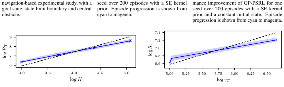
- The empirical horizon dependence in the paper's experiments is closer to H than to the proved H^{3/2}, suggesting the upper bound may be sharpened further.
Reading between the lines
- The Gaussian-noise assumption is the load-bearing premise: Lemma 4.7 and the Pinsker-based reduction from Bellman error to model error are Gaussian-specific. If the noise is misspecified or heavy-tailed, or σ is unknown, the bounded-ball argument and the final regret bound would need new machinery.
- The top-line abstract expression O(H sqrt(gamma_T T)) does not match the theorem's H^{3/2}; the formal claim is Theorem 4.11 with the H^{3/2} factor.
- The same chaining-plus-discretization machinery could plausibly extend to multi-output Gaussian process priors with correlated reward and dynamics, where the effective information gain is smaller and the regret could improve.
- For locally bounded kernels such as the linear kernel, the authors note the visited-state radius may pick up exponential dependence on H unless the algorithm is restricted to stabilizing policies — a natural direction for follow-up work.
Editorial analysis
A structured set of objections, weighed in public.
Referee Report
Summary. The manuscript analyzes GP-PSRL in an episodic MDP with a continuous unbounded state space R^{ds}, a bounded action set, deterministic bounded reward, and Gaussian transition noise with known variance. Under a GP prior on the dynamics whose kernel is bounded and Hölder-continuous, it proves a Bayesian regret bound of order O(H^{3/2} sqrt((ds+da) γ_N(σ², \tilde R) T log T)) for T satisfying (7). The proof has two main parts: (i) a high-probability concentration argument, based on Borell–Tsirelson–Ibragimov–Sudakov and chaining, showing that all visited states lie in a ball of radius O(sqrt(log T)); and (ii) a regret decomposition through a simulation lemma, followed by a bound on the cumulative model estimation error via discretization, an exponential moment inequality for χ² random variables, an elliptical potential lemma, and a chaining argument for the discretization error. The main technical novelties claimed are the treatment of the unbounded state space and the derivation of a √γ_T rate under only Hölder continuity of the kernel.
Significance. If the main result is correct, it resolves three limitations of prior GP-PSRL theory: suboptimal dependence on the maximum information gain, the unbounded-state-space issue, and restrictive smoothness/prior assumptions. The proof is self-contained and does not fit any parameter to data; the high-probability state-concentration lemma is a genuine and reusable contribution. The result is, however, a Bayesian regret bound under an explicit Gaussian-noise/known-σ assumption, so its practical scope is narrower than the abstract suggests. The central asymptotic claim appears sound; the defects I found are local and do not change the rate.
major comments (2)
- [Lemma E.7] The displayed bound "≤7" is numerically false. At α=1, the expression evaluates to sqrt(72) ≈ 8.49 > 7; the chain of inequalities fails at the final step (√3(4+√8)>7). This is a local constant error: replacing 7 by any constant greater than √72 preserves Lemma E.11 and the O(√log T) discretization bound, so the main rate is unaffected. Nevertheless, the lemma as printed is not correct and should be restated and reproved with a valid constant.
- [Theorem 4.11 / Lemma 4.10 proof] The proof of Lemma 4.10 chooses ε = 1/(L^{1/α} T^{2/α}) and then applies Lemmas E.11–E.12, which require ε ≤ (7/(e√8))^{α/2} \tilde R. This condition is not implied by the lower bound (7); it holds only for T sufficiently large relative to \tilde R, L, and the kernel constants. As written, Theorem 4.11 asserts the bound for all T satisfying (7), which is not justified. The claim is asymptotic and can be repaired by adding a 'for sufficiently large T' qualifier or by capping ε; I do not see any effect on the rate.
minor comments (6)
- [Abstract / Section 1] The abstract states a bound of the form \tilde O(H sqrt(γ_T T)) with 'expected information gain', whereas Theorem 4.11 states O(H^{3/2} sqrt(γ_N T log T)) with N = T/H and γ_N the maximum information gain. Please align the abstract with the main theorem and use consistent terminology.
- [Lemma 4.6 statement] The lemma statement writes sup_{x∈R^{ds+da}(R)}; this should read B^{ds+da}(R). Also, the notation γ_{T/H} in Table 1 is introduced without explanation; clarify that it is γ_N with N = T/H.
- [Section 3.3] The assumption that the initial state distribution is ρ = N(0, σ² I) is essential for Lemma 4.7. This restriction should be stated as a modeling limitation in the discussion, since the regret bound does not automatically extend to arbitrary initial distributions.
- [Appendix A.2] Typo: 'occation' should be 'occasion'.
- [Section 5 / Appendix G] The caption of Figure 8 reads 'Mat´ern kernels'; the accent is misrendered. Also, the captions of Figures 7 and 8 refer to 'predicted rate' and 'empirical rate'; it would be helpful to state explicitly that these are log-log slopes of Bayesian regret, not per-trial regret.
- [Lemma D.1 proof] In the martingale concentration step, the sub-Gaussian parameter is 2R_max H, which is fine, but the notation T in the exponent '2T R²_max H² λ²' may confuse because T = NH; consider writing N(H−1) or clarifying that the total number of summands is at most T.
Circularity Check
No significant circularity: the regret bound is derived from stated assumptions and external inequalities; no fitted parameter or self-citation is load-bearing.
full rationale
The derivation chain is self-contained relative to its stated assumptions. The only quantities entering the final regret bound are the horizon H, the dimensions ds and da, the kernel constants C, L, alpha, the known noise variance sigma^2, and the maximum information gain gamma_N(sigma^2, eR), which is a kernel-complexity measure rather than a fitted function of the regret. The ball radius eR is constructed in Lemma 4.7 from a BTIS concentration argument and then reused as the argument of gamma_N; this is a self-consistent choice of scale, not a definitional identification of the predicted quantity with an input. Lemma 4.8 relies on the standard posterior-sampling identity from Osband et al. (2013), and Lemma 4.9 combines that external result with Lemma 1 of Fan & Ming (2021) via Pinsker's inequality; neither is a self-citation. Lemma 4.10 is an original estimation-error bound proved with standard elliptical-potential and chaining tools; its output is an upper bound on an expectation that is not set equal to the target regret by construction. Theorem 4.11 then combines these bounds. The Gaussian-noise and known-variance assumptions are explicit scope conditions in Section 3.3 rather than hidden circular inputs. I also considered the Lemma E.7 constant issue (the final factor 7 is not valid for alpha=1) and the abstract/main-theorem H-dependence mismatch; these are proof/editorial defects and do not make any step equivalent to its own input. No parameter is fitted and no 'prediction' is a renamed regressor, so the circularity score is 0.
Assumptions & free parameters
assumptions (12)
- standard math Gaussian Lipschitz concentration: a 1-Lipschitz function of a standard Gaussian vector is sub-Gaussian (Lemma 4.3, Wainwright Thm 2.26)
- standard math Borell–Tsirelson–Ibragimov–Sudakov inequality for suprema of Gaussian processes (Lemma 4.1)
- standard math Dudley entropy integral bound for expected suprema of Gaussian processes (Lemma 4.2)
- standard math Posterior sampling regret identity (Lemma 4.8, from Osband et al., 2013)
- standard math Pinsker's inequality relating total variation distance to KL divergence (Lemma D.2)
- standard math Elliptical potential lemma for kernel matrices (Lemma E.2, Srinivas et al., 2012)
- standard math Separability of the Gaussian processes used in the proof (Definition A.1)
- domain assumption Gaussian transition noise with known variance and Gaussian initial state (Section 3.3)
- domain assumption Uniformly bounded and Hölder-continuous kernel (Assumptions 3.3 and 3.4)
- domain assumption Bounded action set and bounded known reward (Assumptions 3.1 and 3.2)
- domain assumption Independent zero-mean GP prior for each dynamics component (Section 3.3)
- domain assumption Exact optimal policy oracle for each sampled MDP (Algorithm 1)
Cite this review
Pith. "Pith review of Posterior Sampling Reinforcement Learning with Gaussian Processes for Continuous Control: Sublinear Regret Bounds for Unbounded State Spaces." pith.science (2026). https://pith.science/paper/IWV2N343
@misc{pith2026260308287,
  author       = {Pith},
  title        = {Pith review of: Posterior Sampling Reinforcement Learning with Gaussian Processes for Continuous Control: Sublinear Regret Bounds for Unbounded State Spaces},
  year         = {2026},
  howpublished = {\url{https://pith.science/paper/IWV2N343}},
  note         = {Machine review of arXiv:2603.08287}
}
abstract
We analyze the Bayesian regret of the Gaussian process posterior sampling reinforcement learning (GP-PSRL) algorithm. Posterior sampling is a heuristic for decision-making under uncertainty that has been used to develop successful algorithms for a variety of continuous control problems. However, theoretical work on GP-PSRL is limited. All known regret bounds either have a sub-optimal growth rate, require strong smoothness assumptions, or fail to properly account for the fact that the set of possible system states is unbounded. Through a recursive application of the Borell-Tsirelson-Ibragimov-Sudakov inequality, we show that, with high probability, the states actually visited by the algorithm are contained within a ball of near-constant radius. We then use the chaining method to control the regret suffered by GP-PSRL under weak smoothness conditions. Our main result is a Bayesian regret bound of the order $\widetilde{\mathcal{O}}(H\sqrt{\gamma_TT})$, where $H$ is the horizon, $T$ is the number of time steps and $\gamma_T$ is the expected information gain. With this result, we resolve the limitations with prior theoretical work on PSRL, and provide the theoretical foundation and tools for analyzing PSRL in complex settings.
Figures


Figures from the paper (1 more)
Reference graph
Works this paper leans on
-
[1]
Thus we have R1 = max(2σ p ds, p 16σ2 log(T))≤168α −1/2p max(C, σ2)(ds +d a) log(10(T+R a) max(1, L/C))
First, we have 2σ p ds ≤2α −1/2p max(C, σ2)(ds +d a) log(10(T+R a) max(1, L/C)) Next, we have p 16σ2 log(T)≤4α −1/2p max(C, σ2)(ds +d a) log(10(T+R a) max(1, L/C)). Thus we have R1 = max(2σ p ds, p 16σ2 log(T))≤168α −1/2p max(C, σ2)(ds +d a) log(10(T+R a) max(1, L/C)). 23 Posterior Sampling Reinforcement Learning with Gaussian Processes for Continuous Con...
2013
-
[2]
Tail Bounds for Suprema of Gaussian Processes We prove the results given in Section 4.2
B. Tail Bounds for Suprema of Gaussian Processes We prove the results given in Section 4.2. In Appendix B.1, we prove Lemma 4.5 and we use bounds on the covering number and diameter of Bds+da (R) w.r.t dc to obtain an explicit upper bound for the expected supremum. In Appendix B.2, we prove Lemma 4.4. Finally, in Appendix B.3, we prove Lemma 4.6. B.1. Exp...
2019
-
[3]
lim n→∞ sup x∈Z (n) ∥f(x)∥ 2 # = lim n→∞ E
By introducing a telescoping sum and then using the triangle inequality, we obtain E sup x∈Z ∥f(x)∥ 2 =E sup x∈Z ∥f(x)∥ 2 −sup x∈Z ∥f(ω m(x))∥2 +E[∥f(x 0)∥2] + mX k=k+0+1 E sup x∈Z ∥f(ω k(x))∥2 −sup x∈Z ∥f(ω k−1(x))∥2 ≤E sup x∈Z ∥f(x)−f(ω m(x))∥2 +E[∥f(x 0)∥2] + mX k=k0+1 E sup x∈Z ∥f(ω k(x))−f(ω k−1(x))∥2 . Since Z is finite, we can choose m to be large ...
2014
-
[5]
I{A} NX n=1 V Mn πn,1 (sn,1)−V M⋆ πn,1(sn,1) # ≤E
Fortunately, one can still upper bound this expected value by a quantity that turns out to be negligible compared to the dominant term of the final regret bound. Lemma D.1.For any eventA, E " I{A} NX n=1 V Mn πn,1 (sn,1)−V M⋆ πn,1(sn,1) # ≤E " I{A} NX n=1 H−1X h=1 ⟨P (n) n,h −P ⋆ n,h, VMn πn,h+1⟩ # + 2RmaxH √ 2πT . Proof.First, we use the Bellman equation...
2021
-
[6]
Using Lemma E.2, one can prove a version of the elliptical potential lemma that accounts for the fact that f (n) is only re-sampled at the end of each episode
log det 1 σ2 CT +I . Using Lemma E.2, one can prove a version of the elliptical potential lemma that accounts for the fact that f (n) is only re-sampled at the end of each episode. The result below is proved in the proof of Theorem 1 in Fan & Ming (2021). Lemma E.3.With probability 1, I{A} NX n=1 H−1X h=1 σ2 n−1(xn,h)≤ 2CH log(1 +C/σ
2021
-
[2014]
Huang, K., Kakade, S. M., Lee, J. D., and Lei, Q. A short note on the relationship of information gain and eluder dimension.arXiv preprint arXiv:2107.02377,
Reviewed August 2, 2026 · model on record in the stance chip above.
Discussion (0). Continue with ORCID to comment.