REVIEW 3 major objections 6 minor 13 references
Regression Adjustments for Double Randomization in Two-Sided Marketplaces
T0 review · 3 major / 6 minor · reviewed 2026-07-13 · grok-4.5
Pith's one-line read Optimal regression adjustments for two-sided marketplace experiments can be estimated from observed data alone and beat classical ANCOVA without assuming a linear model.
desk verdict Solid, usable extension of Lin/ToM-style adjustment to MRD marketplace designs; the optimal coefficients are estimable and the theory is careful. read the letter →
The pith
A machine-rendered reading of the paper's core claim, the machinery that carries it, and where it could break.
The reading
What carries the argument
The non-interacted imputation estimator τ̂_c(β) together with the estimable quadratic form Z̃_c, ũ_c built from buyer-mean, seller-mean, and double-decentered residual moments; minimizing that form yields the optimal β̃_c that can be plugged in from data.
What would settle it
In a large-scale MRD with known ground-truth effects, compute the optimal plug-in estimator and ordinary ANCOVA on the same covariates; if the plug-in fails to reduce empirical variance relative to ANCOVA (or the unadjusted estimator) once treatment fractions become unbalanced, the optimality claim is falsified.
Extended reading notes
Core claim
Among the class of non-interacted linear imputation estimators for any linear combination of the four cell means, the asymptotic-variance-minimizing coefficient is estimable from observed data by plugging empirical double-decentered moments into the quadratic form that defines the population variance; the resulting plug-in is model-robustly consistent and asymptotically normal for the true finite-population effect.
Load-bearing premise
The variance of the optimally adjusted estimator must scale like one over the number of buyers (or one over the product of buyers and sellers for the pure direct-effect case) and the associated Gram matrices must stay invertible; if row or column variation vanishes faster, consistency and the confidence intervals can fail.
Signed reviews
Editorial analysis
A structured set of objections, weighed in public.
Referee Report
Summary. The paper develops model-robust regression adjustments for Multiple Randomization Designs (MRDs) in two-sided marketplaces. Among non-interacted linear imputation estimators of the form τ̂_c(β)=∑_γ c_γ (1/(I_γ J_γ)) ∑_{(i,j)∈γ}(y_ij−X_ij^ opβ), it derives the asymptotic-variance-minimizing coefficient β̃_c as the solution of an explicit positive-definite quadratic form whose Gram and cross-moment matrices are population moments of covariates and potential outcomes. These matrices are estimable from within-cell double-decentered sample moments, yielding a plug-in estimator that is asymptotically normal for the finite-population target τ_c without any linearity assumption on potential outcomes (Theorem 3.1, Propositions 3.1–3.2). For the direct effect the plug-in coincides with a weighted interacted two-way fixed-effects regression; for total and spillover effects the optimal adjustment is generally not a simple OLS form. The paper also supplies improved Wasserstein CLTs and consistent conservative variance estimators for doubly-randomized sums, and demonstrates efficiency gains over unadjusted and ANCOVA estimators in simulations.
Significance. If the results hold, the paper supplies the natural design-based analogue of Lin/ToM-style regression adjustment for marketplace experiments under local interference—an important practical gap, since MRDs often suffer from low power when one side of the market is small. The derivation that the optimal coefficient is identifiable from observed double-decentered moments alone, without unobservable potential-outcome contrasts, is non-obvious and useful. The improved finite-population CLT for doubly-randomized sums (Theorem 3.3) and the accompanying variance-consistency result (Theorem 3.4) are of independent interest and relax boundedness and θ(I^{-1}) lower-bound assumptions used in prior MRD theory. Simulations show material efficiency gains, especially in imbalanced designs. The work is carefully situated relative to Freedman, Lin, Li–Ding, and Lu–Liu, and the finite-population randomization framework is rigorous.
major comments (3)
- Assumption 4 (and the companion lower bound used for the improved CLT) is load-bearing for plug-in consistency of β̂_c and for validity of the conservative intervals (Propositions 3.1–3.2, Theorem 3.2). The paper correctly isolates the direct-effect θ((IJ)^{-1}) regime in Example 3.1 and flags multi-regime theory as open (Introduction, §5). For a methods paper aimed at practitioners, however, the manuscript should give clearer operational guidance: how an experimenter can diagnose whether buyer/seller-mean variation is of order θ(1) versus o(1), and what fails (and what still works) when the Gram matrix I∑_γ a_γ,θ Z_θ is nearly singular. Without that, the scope of the main inferential guarantees is hard to assess from data alone.
- Section F derives optimal interacted imputation coefficients for direct, total, and spillover effects and reports a simulation (Figure 6) in which the optimal interacted estimator substantially outperforms Lin-style separate OLS. The abstract and §1.3 list interacted estimators among the contributions, yet asymptotic normality, plug-in consistency, and inference for the interacted class are deferred. Either complete the parallel theory (the non-interacted arguments appear to extend) or clearly relegate interacted estimators to an exploratory appendix so that the main claims match the proved results.
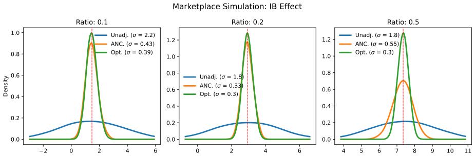
- Section 4 (Figures 3 and 5): the optimal adjustment reduces Monte Carlo variance more than it shortens the conservative confidence intervals, and all methods overcover. The text notes this briefly but does not quantify how much of the efficiency gain is lost to the Cauchy–Schwarz-style bound V_c of [MVR+24]. Because the paper’s practical selling point is “better inference when running MRDs,” a short analysis of when the plug-in residual variance estimator remains substantially conservative after optimal adjustment would strengthen the inferential claims.
minor comments (6)
- Table 1 is helpful but the “∼ (Direct Effect)” entry for non-interacted regression form is slightly cryptic; a one-sentence clarification in the table note would help.
- Notation for group sizes I_γ, J_γ versus I_T, I_C is introduced gradually; a short notation paragraph early in §1.5 would reduce friction.
- In the direct-effect WLS representation (Eq. 6 and Appendix B), the full list of identifiability constraints is long; stating that they force within-group double-decentering would make the equivalence more transparent.
- Figure 1 and the simulation legends use “σ =” for estimated standard deviations; labeling them as Monte Carlo SDs would avoid confusion with the theoretical σ_Tot.
- A few typos and typesetting issues remain (e.g., “/leftr↦g⊳tl↦ne” artifacts in Theorem 3.4 and related displays; “I ∑_γ a_γ,θ Z_θ” in Assumption 4).
- The discussion of switchback and clustered MRD extensions (§1.4) is interesting but could be shortened or moved to the discussion to keep the main narrative focused.
Circularity Check
No significant circularity: optimal coefficients minimize an explicit finite-population variance quadratic form; the plug-in replaces population moments by within-cell sample analogues, and asymptotic claims are proved from first principles.
full rationale
The paper’s central derivation is self-contained and non-circular. The class of non-interacted imputation estimators is defined explicitly (Eq. 7 / 16). Their design-based variance is expanded via the Hoeffding decomposition of doubly randomized group means (Propositions A.1–A.2, Appendix A) into a positive-definite quadratic form β⊺Z̃_c β − 2ũ_c⊺β + C, where Z̃_c and ũ_c are linear combinations of double-decentered Gram and cross-moment matrices of the fixed potential outcomes and covariates. The optimal coefficient is the FOC solution β̃_c = Z̃_c^{-1}ũ_c; the plug-in replaces those population moments by within-cell sample analogues (Eqs. 22–25). Consistency of the plug-in, asymptotic equivalence of oracle and plug-in estimators, and the CLT (Theorem 3.1, Propositions 3.1–3.2) are proved under stated finite-population regularity conditions, using a new Wasserstein CLT for doubly randomized sums derived in the paper (Theorem 3.3) rather than imported as an unexamined black box. Self-citations to MVR+24 / BBI+21 supply the MRD design and unadjusted baseline; they are not load-bearing for the optimality or model-robustness claims. No fitted parameter is later re-labeled a prediction, no uniqueness theorem is smuggled in, and no known empirical pattern is merely renamed. Score 0 is therefore appropriate.
Assumptions & free parameters
assumptions (4)
- domain assumption Local interference: y_ij(W) depends on W only through the pair treatment W_ij and the two fractions of treated partners for i and for j (Definition 1.1).
- domain assumption Finite-population limits of the second-moment matrices heta_ au, u_ au^ heta, Z^ heta exist and are finite (Assumption 1).
- ad hoc to paper Variance lower bound Var( aû_c(etã_c)) = heta(I^{-1}) (or heta((IJ)^{-1}) for direct effect) together with invertibility of the limiting Gram matrices (Assumption 4).
- domain assumption Completely randomized assignment of buyer and seller indicators with fixed margins I_T, J_T (simple MRD).
Cite this review
Pith. "Pith review of Regression Adjustments for Double Randomization in Two-Sided Marketplaces." pith.science (2026). https://pith.science/paper/7KCSK52G
@misc{pith2026260319480,
  author       = {Pith},
  title        = {Pith review of: Regression Adjustments for Double Randomization in Two-Sided Marketplaces},
  year         = {2026},
  howpublished = {\url{https://pith.science/paper/7KCSK52G}},
  note         = {Machine review of arXiv:2603.19480}
}
read the original abstract
Multiple randomization designs (MRDs) are a class of experimental designs used to handle interference in two-sided marketplaces. We investigate regression adjustment strategies for estimating total, spillover, and direct effects in MRDs. We derive minimum asymptotic variance estimators among a broad class of linearly adjusted estimators, without assuming a linear model on the potential outcomes. Surprisingly, the optimal regression adjustments are estimable from data and are generally different from regression adjustments in classical randomized experiments. For example, one such optimal estimator for the direct effect corresponds to a weighted regression with interacted two-way fixed effects. We establish model-robustness properties, central limit theorems, and inferential methods for our estimators, relying on improved theoretical results for MRD experiments. Our results provide the analog of classical regression adjustments for marketplace experiments. Numerical simulations demonstrate a considerable increase in efficiency over simpler approaches, enabling better inference when running MRDs.
Figures


Figures from the paper (3 more)


Reference graph
Works this paper leans on
-
[1]
Design and analysis of switchback experiments
7, 8 [BSLZ23] Iavor Bojinov, David Simchi-Levi, and Jinglong Zhao. Design and analysis of switchback experiments. Management Science, 69(7):3759–3777, 2023. 8 24 [CF24] Peter L Cohen and Colin B Fogarty. No-harm calibration for generalized oaxaca–blinder estimators. Biometrika, 111(1):331–338, 2024. 16, 24 [Din24] Peng Ding. A first course in causal infer...
2023
-
[2]
On regression adjustments to experimental data
8, 20 [Fre08b] David A Freedman. On regression adjustments to experimental data. Advances in Applied Mathematics, 40(2):180–193, 2008. 4, 5, 8, 20 [GB23] Kevin Guo and Guillaume Basse. The generalized oaxaca-blinder estimator. Journal of the American Statistical Association, 118(541):524–536, 2023. 9, 24 [Gol07] Larry Goldstein. l 1 bounds in normal appro...
arXiv 2008
-
[3]
For (77), Lemma D.1 gives us the upper bound 1 I2 I ∑ i=1 Var(ˆ¯yi,●)2≲1 I2 I ∑ i=1 ⎡⎢⎢⎢⎢⎣ 1 J2 J ∑ j=1 (yij−yi,●)2 ⎤⎥⎥⎥⎥⎦ 2 ≲1 I5 ∑ i,j (yij−yi,●)4 ≲1 I5 ∑ i,j (yij−yi,●)2⋅max∣yi,●−yij∣2 ≲1 I Var(ˆ¯¯y)⋅max∣yi,●−yij∣2 48
-
[4]
For (78), applying the same subgaussian moment bound and Jensen’s inequality yields 1 I2 I ∑ i=1 E[(̂yi,●−yi,●) 3 ](yi,●−¯¯y) ≲max i ∣yi,●−¯¯y∣1 I2 I ∑ i=1 ⎡⎢⎢⎢⎢⎣ 1 J2 J ∑ j=1 (yij−yi,●)2 ⎤⎥⎥⎥⎥⎦ 3/2 ≲max i ∣yi,●−¯¯y∣ 1 I2J3/2J ∑ i,j ∣yij−yi,●∣3 ≲1 I1/2max i ∣yi,●−¯¯y∣max ij ∣yij−yi,●∣Var[ˆ¯¯y]
-
[5]
For (79) apply the same logic: 1 I2 I ∑ i=1 E[(̂yi,●−yi,●) 2 ](yi,●−¯¯y) 2 ≲max i ∣yi,●−¯¯y∣2 1 I2 I ∑ i=1 ⎡⎢⎢⎢⎢⎣ 1 J2 J ∑ j=1 (yij−yi,●)2 ⎤⎥⎥⎥⎥⎦ ≲max i ∣yi,●−¯¯y∣2 Var(ˆ¯¯y)
-
[6]
For (80), we can easily upper bound the term by 1 I ωB(yij)max i∣yi,●−¯¯y∣2 ≤Var(ˆ¯¯y)maxi∣yi,●− ¯¯y∣2. Combining the individual bounds gives the upper bound 1 I2 I−2∑I i=1 E[(̂yi,●−¯¯y) 4 ] Var(ˆ¯¯y)2 ≲1 I3 maxij ∣yij−yi,●∣2 Var(ˆ¯¯y) + 1 I5/2 maxi∣yi,●−¯¯y∣maxij ∣yij−yi,●∣ Var(ˆ¯¯y) + 1 I2 maxi∣yi,●−¯¯y∣2 Var(ˆ¯¯y) Under the given assumptions, the expre...
-
[7]
The variance of the direct effect estimator is Θ(1/IJ)
-
[8]
Asymptotic normality of ˆτdir(ˆτdir)
Show all 13 references
-
[9]
For the first claim, it suffices to proveω θ(eij(γ))=O(1/I)and alsoξ θ γ,γ ′ =O(1/I)forθ∈{B,S}
Asymptotically conservative confidence intervals using the plug-in. For the first claim, it suffices to proveω θ(eij(γ))=O(1/I)and alsoξ θ γ,γ ′ =O(1/I)forθ∈{B,S}. Sinceξ θ γ,γ ′ ≲ωθ γ+ω θ γ′,we need only proveω θ(eij(γ))=O(1/I). Expand ωθ(eij(γ))=β ⊺ dirZθβdir−2u⊺ γβdir+ω θ γ...
-
[10]
Using the covariance formula for sampling without replacement, this is upper bounded by a constant multiple times 1 IJ 2 ∑ i,j (aij−¯ai,●)(b ij−¯bi,●)
For the first term (94), the mean is given by 1 I ∑I i=1 Cov(ˆ¯ai,●,ˆ¯bi,●)using the tower property. Using the covariance formula for sampling without replacement, this is upper bounded by a constant multiple times 1 IJ 2 ∑ i,j (aij−¯ai,●)(b ij−¯bi,●). Applying Cauchy-Schwarz ...
-
[11]
Thus it suffices to compute the variance
For the second term (95), conditioning onBshows that the expression is mean zero. Thus it suffices to compute the variance. Using the law of total variance and conditioning on the buyer variables, the variance is given by E ⎡⎢⎢⎢⎢⎣ Var ⎡⎢⎢⎢⎢⎣ 1 Iγ ∑ i∈Iγ ¯a(d) i,● ˆ¯bi,●∣B ⎤⎥⎥⎥...
-
[12]
The third term is symmetric to the second term and isO p(( 1 I ωB(b)) 1/2 )
-
[13]
Note that Var⎛ ⎝ 1 Iγ ∑ i∈Iγ ¯a(d) i,● ¯b(d) i,● ⎞ ⎠≲1 I2 I ∑ i=1 (¯ai,●−¯¯a)2(¯bi,●−¯¯b)2 ≤1 I max i (¯bi,●−¯¯b)2 1 I I ∑ i=1 (¯ai,●−¯¯a)2 ≤1 I max i (¯bi,●−¯¯b)2ωB(a)
For the last term, bound it above byO p( √ Var( 1 Iγ ∑i∈Iγ ¯a(d) i,● ¯b(d) i,●)). Note that Var⎛ ⎝ 1 Iγ ∑ i∈Iγ ¯a(d) i,● ¯b(d) i,● ⎞ ⎠≲1 I2 I ∑ i=1 (¯ai,●−¯¯a)2(¯bi,●−¯¯b)2 ≤1 I max i (¯bi,●−¯¯b)2 1 I I ∑ i=1 (¯ai,●−¯¯a)2 ≤1 I max i (¯bi,●−¯¯b)2ωB(a). We could have equivalentl...
2000
Reviewed July 13, 2026 · model on record in the stance chip above.
Discussion (0). Continue with ORCID to comment.