REVIEW 2 major objections 4 minor 21 references
Achieving $\widetilde{O}(1/\epsilon)$ Sample Complexity for Bilinear Systems Identification under Bounded Noises
T0 review · 2 major / 4 minor · reviewed 2026-07-13 · grok-4.5
Pith's one-line read Set-membership identification of bilinear systems under bounded noise reaches Õ(1/ε) sample complexity, even with trajectory-dependent regressors and only polynomial mean-square growth.
desk verdict Solid extension of the optimal bounded-noise SME rate to bilinear systems; the math holds under the stated assumptions and the main soft spot is the boundary-mass condition already flagged. read the letter →
The pith
A machine-rendered reading of the paper's core claim, the machinery that carries it, and where it could break.
The reading
What carries the argument
The feasible-parameter set S_T (equivalently its error counterpart Γ_T) whose diameter is controlled by a block-wise excitation event derived from a one-step block-martingale small-ball condition on the bilinear regressor, combined with a geometric elimination argument that uses the noise’s boundary mass.
What would settle it
Simulate a marginally stable bilinear system whose noise is bounded and symmetric but has vanishing density near the support boundary (e.g., a truncated density that approaches zero at the edge); if the measured diameter of the set-membership set then decays only as 1/√T or slower, the claimed rate is false under the stated assumptions.
Extended reading notes
Core claim
Under i.i.d. bounded inputs, bounded symmetric log-concave disturbances that put linear mass near the boundary of their support, and the mild spectral-radius condition that yields only polynomial mean-square state growth, the diameter of the set-membership feasible set for a discrete-time bilinear system contracts with sample complexity Õ(1/ε). The same linear rate previously obtained for linear systems therefore extends to the bilinear class without requiring asymptotic stability.
Load-bearing premise
The noise must put at least linear probability mass in every thin shell near the boundary of its known bound; if that mass vanishes faster than linear, the 1/ε contraction fails.
Editorial analysis
A structured set of objections, weighed in public.
Referee Report
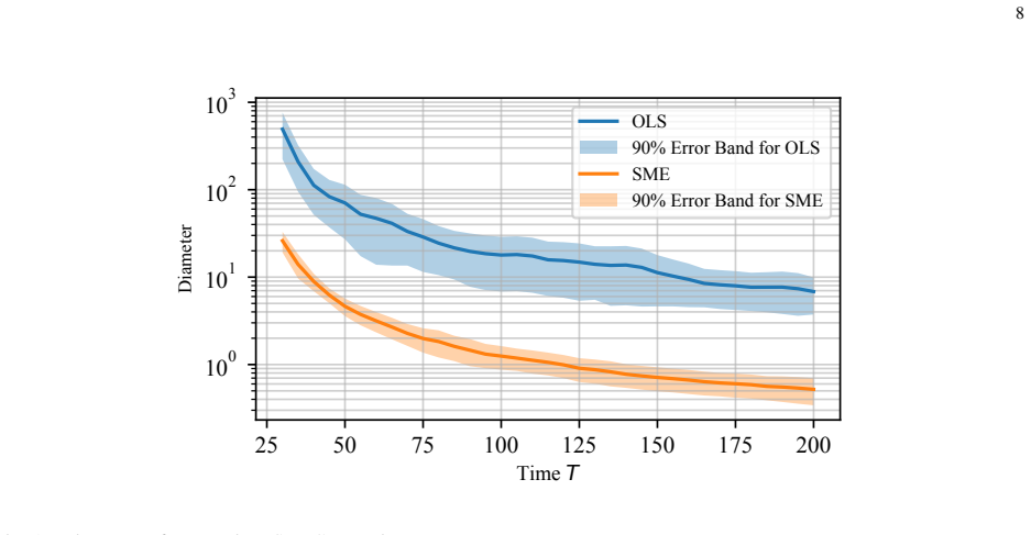
Summary. The paper develops a finite-sample set-membership identification (SME) analysis for discrete-time bilinear systems under bounded, symmetric, log-concave noise. The system is written as x_{t+1}=Θ⋆ z_t + w_t with trajectory-dependent regressor z_t = [x_t; u_t ⊗ x_t]. Under i.i.d. bounded inputs (Ass. 1), bounded log-concave noise (Ass. 2), and a linear boundary-mass condition on the noise (Ass. 3), the authors prove that the diameter of the SME feasible set S_T contracts with sample complexity Õ(1/ε). The argument proceeds via three main lemmas: polynomial mean-square state growth under ρ(Ã)≤1 (Lemma 1), a BMSB condition for z_t under log-concave noise via Paley–Zygmund and moment comparison (Lemma 2), and block-wise elimination of large parameter errors using covering numbers plus boundary mass (Lemmas 3 and 6). Theorem 1 gives an explicit (implicitly logarithmic) sample bound. Simulations compare SME diameters to OLS 90% confidence regions on a structured marginally stable bilinear example.
Significance. The result closes a natural gap between recent Õ(1/ε) SME rates for linear systems under bounded noise and existing least-squares analyses of bilinear systems. Allowing trajectory-dependent regressors and only polynomial mean-square growth (rather than asymptotic stability) is a genuine technical contribution relative to both the linear SME literature and the general analytic-system result of [20]. The appendices supply complete proofs of the growth, BMSB, and elimination steps, and the authors release simulation code. If the boundary-mass assumption is accepted as standard for set-membership rates, the paper provides a clean, dimension-explicit guarantee that is useful for uncertainty quantification in bilinear control applications.
major comments (2)
- Assumption 3 (boundary mass) is load-bearing for the claimed Õ(1/ε) rate. Lemma 6 obtains geometric decay of P(E_1 ∩ E_2) only because each excited block forces a boundary hit of probability ≥ q_w(ε_δ) ∝ ε_δ; without the linear lower bound the elimination argument yields a weaker rate. The manuscript should state this dependence more prominently (e.g., in the statement of Theorem 1 or the discussion after it) and note that the rate can fail for noise distributions that put vanishing mass near ∂W, even if they remain bounded and log-concave.
- Theorem 1, display (16): the sample bound is written with T appearing on both sides (log T terms). While this is common, the paper claims an explicit Õ(1/ε) guarantee. A short remark converting (16) into a fully explicit T ≥ C log(C/η)/δ form (or an iterative bound) would make the main claim easier to cite and compare with [15], [20].
minor comments (4)
- Lemma 1: the Jordan argument gives r = n^{2} (or d = n^{2}), yet the text later writes r ∈ {0,…,n-1}. Align the exponent with the dimension of the second-moment map.
- Simulation (Fig. 1): the SME diameter is approximated by a non-convex surrogate as in [15]. A one-sentence description of the approximation (or a pointer to the code) would help reproducibility.
- Notation: the same symbol ε is used for estimation error, covering radius, and boundary thickness; a short glossary or consistent subscripts would reduce ambiguity.
- Typos: title/abstract use both Õ and eO; “BMSM condition” appears once in the appendix; “vec(Σ_t)” formatting is occasionally inconsistent.
Circularity Check
No circularity: Õ(1/ε) diameter contraction is derived from BMSB, covering, and boundary-mass assumptions, not from fitted inputs or load-bearing self-definition.
full rationale
The central claim (Theorem 1) is a non-asymptotic high-probability bound on diam(S_T). Its proof reduces diam(S_T) to diam(Γ_T), splits on the block-excitation event E_2, and bounds P(E_2^c) and P(E_1 ∩ E_2) via Lemmas 3 and 6. Those lemmas rest on: (i) polynomial mean-square growth of x_t from the variance recursion under ρ(Ã)≤1 (Lemma 1); (ii) a (1,k_z²I,p_z)-BMSB property for the bilinear regressor under symmetric log-concave noise, proved with Paley–Zygmund and fourth-moment comparison (Lemma 2); (iii) standard ε-net covering and small-ball lower tails (Lemmas 4–5, the latter from external [4]); and (iv) geometric elimination of large errors using Assumption 3’s linear boundary mass. None of these steps defines the target diameter in terms of itself, fits a free parameter to data and re-labels it a prediction, or imports a uniqueness theorem that forces the rate. Citations to prior SME/bilinear work ([15], [16], [20]) supply background tools and comparisons; the covering-number restatement from [15] is a standard geometric fact, not a self-justifying premise of the Õ(1/ε) claim. The implicit T-on-both-sides form of (16) is ordinary Õ bookkeeping. Simulation diameter surrogates do not enter the proof. Conclusion: the derivation is self-contained against its stated assumptions; circularity score 0.
Assumptions & free parameters
free parameters (2)
- BMSB constants (k_z, p_z)
- boundary-mass constant c_w and polynomial-growth constants (c_PMS, r, C_z)
assumptions (5)
- domain assumption Input process is i.i.d., zero-mean, coordinate-wise bounded, and has isotropic covariance σ_u² I (Assumption 1).
- domain assumption Noise is i.i.d., zero-mean, supported on the ∞-ball of radius w_max, and every one-dimensional marginal is symmetric and log-concave (Assumption 2).
- domain assumption Boundary-mass lower bound: P(b w_t[j]≥w_max−ε)≥c_w ε for small ε (Assumption 3).
- domain assumption Spectral radius of the second-moment map à satisfies ρ(Ã)≤1, implying polynomial mean-square state growth of degree at most n²−1 (Lemma 1).
- standard math Standard tools: Paley–Zygmund inequality, ε-net covering numbers of the unit sphere, Jordan-block bounds on ‖Ã^t‖, and the block-martingale small-ball lemma of Simchowitz et al.
Cite this review
Pith. "Pith review of Achieving $\widetilde{O}(1/\epsilon)$ Sample Complexity for Bilinear Systems Identification under Bounded Noises." pith.science (2026). https://pith.science/paper/Q4QQHXFT
@misc{pith2026260320819,
  author       = {Pith},
  title        = {Pith review of: Achieving $\widetildeO(1/\epsilon)$ Sample Complexity for Bilinear Systems Identification under Bounded Noises},
  year         = {2026},
  howpublished = {\url{https://pith.science/paper/Q4QQHXFT}},
  note         = {Machine review of arXiv:2603.20819}
}
abstract
This paper studies finite-sample set-membership identification for discrete-time bilinear systems under bounded symmetric log-concave disturbances. Our analysis considers trajectory-dependent regressors and allows marginally stable dynamics with polynomial mean-square state growth. We prove that the diameter of the feasible parameter set shrinks with sample complexity $\widetilde{\mathcal O}(1/\epsilon)$ where $\epsilon$ is the estimation error. Simulation supports the theory and illustrates the advantage of the proposed estimator for uncertainty quantification.
Figures
Reference graph
Works this paper leans on
-
[20]
Identification of analytic nonlinear dynamical systems with non-asymptotic guarantees,
N. Musavi, Z. Guo, G. Dullerud, and Y . Li, “Identification of analytic nonlinear dynamical systems with non-asymptotic guarantees,” inAdvances in Neural Information Processing Systems(A. Globerson, L. Mackey, D. Belgrave, A. Fan, U. Paquet, J. Tomczak, and C. Zhang, eds.), vol. 37, pp. 85500–85522, Curran Associates, Inc., 2024
2024
-
[15]
Learning the uncertainty sets of linear control systems via set membership: a non-asymptotic analysis,
Y . Li, J. Yu, L. Conger, T. Kargin, and A. Wierman, “Learning the uncertainty sets of linear control systems via set membership: a non-asymptotic analysis,” inProceedings of the 41st International Conference on Machine Learning, ICML’24, JMLR.org, 2024
2024
-
[1]
Near optimal finite time identification of arbitrary linear dynamical systems,
T. Sarkar and A. Rakhlin, “Near optimal finite time identification of arbitrary linear dynamical systems,” inProceedings of the 36th International Conference on Machine Learning(K. Chaudhuri and R. Salakhutdinov, eds.), vol. 97 ofProceedings of Machine Learning Research, pp. 5610–5618, PMLR, 09–15 Jun 2019
2019
-
[2]
Non-asymptotic identification of lti systems from a single trajectory,
S. Oymak and N. Ozay, “Non-asymptotic identification of lti systems from a single trajectory,” in2019 American Control Conference (ACC), pp. 5655–5661, 2019
2019
-
[3]
System identification under bounded noise: Optimal rates beyond least squares,
X. Zeng, J. Yu, and N. Ozay, “System identification under bounded noise: Optimal rates beyond least squares,”IEEE Control Systems Letters, vol. 9, pp. 1087–1092, 2025
2025
-
[4]
Learning without mixing: Towards a sharp analysis of linear system identification,
M. Simchowitz, H. Mania, S. Tu, M. I. Jordan, and B. Recht, “Learning without mixing: Towards a sharp analysis of linear system identification,” inProceedings of the 31st Conference On Learning Theory(S. Bubeck, V . Perchet, and P. Rigollet, eds.), vol. 75 ofProceedings of Machine Learning Research, pp. 439–473, PMLR, 06–09 Jul 2018
2018
-
[5]
Naive exploration is optimal for online lqr,
M. Simchowitz and D. Foster, “Naive exploration is optimal for online lqr,” inProceedings of the 37th International Conference on Machine Learning(H. D. III and A. Singh, eds.), vol. 119 ofProceedings of Machine Learning Research, pp. 8937–8948, PMLR, 13–18 Jul 2020
2020
-
[6]
Convergence properties of the membership set,
E.-W. Bai, H. Cho, and R. Tempo, “Convergence properties of the membership set,”Automatica, vol. 34, no. 10, pp. 1245– 1249, 1998
1998
Show all 21 references
-
[7]
The size of the membership-set in a probabilistic framework,
H. Akc ¸ay, “The size of the membership-set in a probabilistic framework,”Automatica, vol. 40, no. 2, pp. 253–260, 2004
2004
-
[8]
Set membership identification of nonlinear systems,
M. Milanese and C. Novara, “Set membership identification of nonlinear systems,”Automatica, vol. 40, no. 6, pp. 957–975, 2004
2004
-
[9]
On the sample complexity of set membership estimation for linear systems with disturbances bounded by convex sets,
H. Xu and Y . Li, “On the sample complexity of set membership estimation for linear systems with disturbances bounded by convex sets,” in2025 American Control Conference (ACC), pp. 3856–3862, IEEE, 2025
2025
-
[10]
Closure: Fast quantification of pose uncertainty sets,
Y . Gao, Y . Tang, H. Qi, and H. Yang, “Closure: Fast quantification of pose uncertainty sets,”arXiv preprint arXiv:2403.09990, 2024
2024 arXiv
-
[11]
Set membership identification of linear systems with guaranteed simulation accuracy,
M. Lauricella and L. Fagiano, “Set membership identification of linear systems with guaranteed simulation accuracy,”IEEE Transactions on Automatic Control, vol. 65, no. 12, pp. 5189–5204, 2020
2020
-
[12]
Online learning of stabilizing controllers using noisy input-output data and prior knowledge,
N. Niknejad, F. A. Yaghmaie, and H. Modares, “Online learning of stabilizing controllers using noisy input-output data and prior knowledge,”IEEE Open Journal of Control Systems, 2025. 15
2025
-
[13]
Online adversarial stabilization of unknown networked systems,
J. Yu, D. Ho, and A. Wierman, “Online adversarial stabilization of unknown networked systems,”Proceedings of the ACM on Measurement and Analysis of Computing Systems, vol. 7, no. 1, pp. 1–43, 2023
2023
-
[14]
Dual adaptive mpc using an exact set-membership reformulation,
A. Parsi, D. Liu, A. Iannelli, and R. S. Smith, “Dual adaptive mpc using an exact set-membership reformulation,”IFAC- PapersOnLine, vol. 56, no. 2, pp. 8457–8463, 2023
2023
-
[16]
Finite sample identification of bilinear dynamical systems,
Y . Sattar, S. Oymak, and N. Ozay, “Finite sample identification of bilinear dynamical systems,” in2022 IEEE 61st Conference on Decision and Control (CDC), pp. 6705–6711, 2022
2022
-
[17]
Bilinear model predictive control of a hvac system using sequential quadratic programming,
A. Kelman and F. Borrelli, “Bilinear model predictive control of a hvac system using sequential quadratic programming,” IFAC Proceedings Volumes, vol. 44, no. 1, pp. 9869–9874, 2011. 18th IFAC World Congress
2011
-
[18]
Finite sample identification of partially observed bilinear dynamical systems,
Y . Sattar, Y . Jedra, M. Fazel, and S. Dean, “Finite sample identification of partially observed bilinear dynamical systems,” 2025
2025
-
[19]
Mean square stability conditions for discrete stochastic bilinear systems,
C. Kubrusly and O. Costa, “Mean square stability conditions for discrete stochastic bilinear systems,”IEEE Transactions on Automatic Control, vol. 30, no. 11, pp. 1082–1087, 1985
1985
-
[21]
Moments, concentration, and entropy of log-concave distributions,
A. Marsiglietti and J. Melbourne, “Moments, concentration, and entropy of log-concave distributions,” 2025
2025
Reviewed July 13, 2026 · model on record in the stance chip above.
Discussion (0). Sign in to comment.