Probes of chaos over the Clifford group and approach to Haar values
Pith reviewed 2026-05-13 23:33 UTC · model grok-4.3
The pith
Expectation values of chaos probes match Haar distribution moments for GUE and T-doped circuits but deviate for GDE.
A machine-rendered reading of the paper's core claim, the machinery that carries it, and where it could break.
Core claim
Using isospectral twirling on fixed spectra with random eigenvectors, the expectation values of the probes adhere to moments of the Haar distribution for chaotic behavior modeled by the Gaussian Unitary Ensemble and T-doped circuits, while deviating for the non-chaotic Gaussian Diagonal Ensemble and showing specific behavior on the Toric Code Hamiltonian.
What carries the argument
Isospectral twirling, which fixes the Hamiltonian spectrum and selects eigenvectors randomly, applied across T-doped circuits and random-matrix ensembles.
If this is right
- The probes distinguish chaotic from non-chaotic regimes by whether their averages match Haar moments.
- T-doped circuits provide a tunable family of states interpolating between Clifford and fully random bases.
- Gaussian Diagonal Ensemble spectra yield systematically different probe values from Gaussian Unitary Ensemble spectra.
- The Toric Code supplies a concrete, non-random benchmark for probe behavior outside the two ensembles.
Where Pith is reading between the lines
- The same twirling procedure could be applied to experimental Hamiltonians to test whether observed probe values indicate chaos without requiring full eigenstate tomography.
- Varying the doping level in T-doped circuits might map a quantitative threshold where probes cross from non-Haar to Haar statistics.
- If the modeling is accurate, spectral statistics alone with randomized eigenvectors suffice to reproduce the probe signatures of chaos without simulating full time evolution.
Load-bearing premise
Randomly chosen eigenvectors from a fixed spectrum accurately capture the statistical signatures of chaotic dynamics in actual quantum systems.
What would settle it
Numerical or experimental computation of the same probe expectation values in a many-body system whose eigenstates are known to be fully chaotic and comparison against the reported GUE and Haar averages.
Figures


read the original abstract
Chaotic behavior of quantum systems can be characterized by the adherence of the expectation values of given probes to moments of the Haar distribution. In this work, we analyze the behavior of several probes of chaos using a technique known as Isospectral Twirling [1]. This consists in fixing the spectrum of the Hamiltonian and picking its eigenvectors at random. Here, we study the transition from stabilizer bases to random bases according to the Haar measure by T-doped random quantum circuits. We then compute the average value of the probes over ensembles of random spectra from Random Matrix Theory, the Gaussian Diagonal Ensemble and the Gaussian Unitary Ensemble, associated with non-chaotic and chaotic behavior respectively. We also study the behavior of such probes over the Toric Code Hamiltonian.
Editorial analysis
A structured set of objections, weighed in public.
Referee Report
Summary. The manuscript claims that probes of quantum chaos adhere to the moments of the Haar distribution when applied to T-doped Clifford circuits approaching Haar-random bases and to isospectral twirling over GUE spectra (modeling chaotic behavior), while deviating for GDE spectra (modeling non-chaotic behavior) and exhibiting specific behavior for the Toric Code Hamiltonian.
Significance. If the results hold, the work provides a controlled numerical approach to benchmarking chaos indicators via isospectral twirling and T-doped circuits, which could help distinguish ergodic from non-ergodic regimes in quantum many-body systems and circuits. The use of standard RMT ensembles as external benchmarks is a clear strength, as is the concrete model for the stabilizer-to-Haar transition.
major comments (1)
- [Sections defining the ensembles and isospectral twirling procedure] The central claim that GDE and GUE under isospectral twirling distinguish non-chaotic from chaotic regimes (and that deviations from Haar moments signal non-chaos) is load-bearing. This modeling choice fixes the spectrum while drawing eigenvectors from the Haar measure, decoupling them; however, physical non-chaotic Hamiltonians typically exhibit correlated, non-random eigenvectors (e.g., due to integrability or localization), so the observed GDE deviations may be an artifact of the artificial construction rather than a robust signature. The manuscript should include direct comparisons with actual integrable or localized Hamiltonians to test this.
minor comments (1)
- [Abstract] The abstract refers to 'several probes of chaos' and 'the average value of the probes' without defining the probes or reporting any numerical values, error bars, or specific adherence metrics, which hinders immediate assessment of the results.
Simulated Author's Rebuttal
We thank the referee for their positive evaluation of the significance of our work and for the constructive major comment. We address the point in detail below and outline the revisions we will make to strengthen the manuscript.
read point-by-point responses
-
Referee: [Sections defining the ensembles and isospectral twirling procedure] The central claim that GDE and GUE under isospectral twirling distinguish non-chaotic from chaotic regimes (and that deviations from Haar moments signal non-chaos) is load-bearing. This modeling choice fixes the spectrum while drawing eigenvectors from the Haar measure, decoupling them; however, physical non-chaotic Hamiltonians typically exhibit correlated, non-random eigenvectors (e.g., due to integrability or localization), so the observed GDE deviations may be an artifact of the artificial construction rather than a robust signature. The manuscript should include direct comparisons with actual integrable or localized Hamiltonians to test this.
Authors: We appreciate the referee's careful analysis of the isospectral twirling construction and its implications for distinguishing chaotic and non-chaotic regimes. The procedure is designed precisely to isolate the role of the spectrum by sampling eigenvectors from the Haar measure, allowing a controlled comparison between ensembles whose only difference is the level statistics (Poissonian for GDE versus Wigner-Dyson for GUE). The fact that probes reach Haar moments under GUE but deviate under GDE indicates that spectral statistics alone are sufficient to drive the distinction in this controlled setting. We acknowledge that physical non-chaotic Hamiltonians generally possess correlated eigenvectors, which the GDE does not capture. To address this directly, we will revise the manuscript to include an explicit comparison of the probe values obtained for the Toric Code Hamiltonian (a concrete integrable model with structured, non-random eigenvectors) against the corresponding GDE results. This addition will clarify the extent to which the GDE deviations are representative of physical non-chaotic behavior and will be presented in a new subsection discussing the limitations and strengths of the ensemble modeling. We believe these changes will reinforce rather than weaken the central claims. revision: yes
Circularity Check
No significant circularity; external RMT benchmarks and standard approximations used
full rationale
The paper computes probe expectation values directly on isospectral-twirled Hamiltonians whose spectra are drawn from the standard GDE and GUE ensembles of random-matrix theory (treated as independent external models for non-chaotic vs. chaotic regimes) and whose eigenvectors are chosen Haar-randomly. The T-doped circuit analysis invokes the known approximation of the Clifford+T group to the Haar measure, without any fitting of parameters to the probes themselves or redefinition of the target Haar moments. The Toric Code is examined as a concrete Hamiltonian instance. No equation reduces a claimed prediction to a fitted input by construction, and the single citation to the isospectral-twirling technique supplies a computational method rather than a load-bearing uniqueness theorem or ansatz that would force the central result. The derivation therefore remains self-contained against external benchmarks.
Axiom & Free-Parameter Ledger
axioms (2)
- domain assumption Random matrix ensembles (GDE, GUE) correctly capture non-chaotic and chaotic spectral statistics of quantum Hamiltonians
- domain assumption Isospectral twirling with Haar-random eigenvectors models the approach to chaotic dynamics
Reference graph
Works this paper leans on
-
[1]
E. H. Lieb,Convex trace functions and the wigner-yanase-dyson conjecture, InSelected Papers of E. H. Lieb. Springer Berlin Heidelberg, Berlin, Heidelberg, ISBN 978-3-642-55925-9, doi:10.1007/978-3-642-55925-9_13 (2002)
-
[2]
K. Yanagi,Uncertainty relation on wigner–yanase–dyson skew information, Journal of Mathematical Analysis and Applications365(1), 12 (2010), doi:10.1016/j.jmaa.2009.09.060
-
[3]
Luo,Wigner–yanase skew information and uncertainty relations, Physics Letters A346, 393 (2005)
S. Luo,Wigner–yanase skew information and uncertainty relations, Physics Letters A346, 393 (2005)
work page 2005
- [4]
-
[5]
S. Furuichi,Information quantities, uncertainty relations, and trace inequalities, Journal of Mathematical Physics 50(1) (2009). 32
work page 2009
-
[6]
Luo,Wigner–yanase skew information and uncertainty relations, Physics Letters A320, 73 (2003)
S. Luo,Wigner–yanase skew information and uncertainty relations, Physics Letters A320, 73 (2003)
work page 2003
-
[7]
P . Gibilisco and T. Isola,Wigner–yanase information on quantum state space: The geometric approach, Journal of Mathematical Physics44, 3752 (2003)
work page 2003
- [8]
-
[9]
Luo,Quantum fisher information and entanglement, Letters in Mathematical Physics71, 1 (2005)
S. Luo,Quantum fisher information and entanglement, Letters in Mathematical Physics71, 1 (2005)
work page 2005
-
[10]
S. Furuichi, K. Yanagi and K. Kuriyama,Fundamental properties of the wigner–yanase–dyson information, Journal of Mathematical Physics45(12), 4868 (2004)
work page 2004
-
[11]
S. Furuichi,On generalized entropies and related topics in quantum information theory, Journal of Mathematical Physics47(2) (2006). Appendix A: Permutation operators properties The symmetric group Sk is the group whose elements permute the order of k elements of a set. For instance the group S2 is the group of operations exchanging the order of two elemen...
work page 2006
-
[12]
Let us start with the simplest Gram matrix, the one for the Haar averages
Gram matrices computation In this section we are going to compute the Gram matrices and their (pseudo)inverse. Let us start with the simplest Gram matrix, the one for the Haar averages. Its elements are defined as: Ωπσ = Tr[TπTσ](B1) Let us forst notice that the product TπTσ =T πσ, so that we effectively need to compute traces of single permutation operat...
-
[13]
In this section we briefly report some results in this regard
Weingarten functions and group characters It is possible to compute the Weingarten functions also from the group characters of the symmetric group. In this section we briefly report some results in this regard. The expression of the Weingarten functionsWπσ in terms of the characters of the irreps of the symmetric groupS 4 is given by: Wπ = X λ d2 λ (4!)2 ...
-
[14]
the calculation of ˆR(2)(V ⊗1,1)
Example:computation of the Haar second moment of a unitary operatorV Let us then consider as working example the calculation of the isospectral twirling of a unitary operator of the form V ⊗k,k for k= 1 , i.e. the calculation of ˆR(2)(V ⊗1,1). One has that the symmetric group of order 2 has only two elements, S2 ={I, T (12)} where I is the identity permut...
-
[15]
TheΞMatrix a. Computation of theΞ πσ In order to compute the matrix elementsΞ πσ we start by rewriting the expression as: Ξπσ = X τ∈S 4 W + πτ Tr TσΘ⊗4QΘ†⊗4QTτ −W − πτ Tr TσΘ⊗4Q⊥Θ†⊗4QTτ = X τ∈S 4 W + πτ Tr TσΘ⊗4QΘ†⊗4QTτ −W − πτ Tr TσΘ⊗4 (1−Q) Θ †⊗4QTτ = X τ∈S 4 W + πτ +W − πτ Tr TσΘ⊗4QΘ†⊗4QTτ −W − πτ Tr [TσQTτ](C1) Let us then define the two matricesK (1)...
-
[16]
The MatrixΓ (k) We remind that the matrixΓ (k) πσ is defined as: Γ(k) πσ = X τ∈S 4 Λπτ k−1X i=0 (Ξi)τ σ (C36) The matrixΛis defined as: Λπτ = X σ∈S4 W − πσ Tr TτΘ⊗4QΘ†⊗4Q⊥Tσ (C37) Let us rewrite the expression as: X σ∈S4 W − πσ Tr TτΘ⊗4QΘ†⊗4Q⊥Tσ = X σ∈S4 W − πσ Tr TτΘ⊗4QΘ†⊗4(1−Q)T σ (C38) = X σ∈S4 W − πσ Tr TτΘ⊗4QΘ†⊗4Tσ −W − πσ Tr TτΘ⊗4QΘ†⊗4QTσ (C39) = X ...
-
[17]
The vector⃗ c Let us now compute the components of the vector ⃗ cfor the order k= 2 isospectral twirling. This corresponds to evaluate the traces: Tr TπV ⊗2,2 ,∀π∈S 4 (D1) These traces can be evaluated according to the conjugacy classes of S4.Let us start with the identity permutation : ⃗ cI = Tr IV ⊗2,2 =|Tr[V]| 4 = X i,j,k,ℓ e−i(Ei+Ej −Ek−Eℓ)t =g 4(t)(D...
-
[18]
The vector⃗ q The computation of the components of the vector ⃗ qis similar to the one of the vector ⃗ c, but not as simple. Indeed, the components of the vecotr⃗ qare defined as: ⃗ qπ = Tr TπQV ⊗2,2 (D9) 42 To evaluate these traces, we once again write the unitary V in its diagonal form. Let us then consider a couple of instances, starting from identity ...
-
[19]
The three point spectral form factorg 3(t) Let us first note that in any computation only the real part of g3(t) will appear, so that we can limit ourselves to average onlyReg 3(t). First of all, we rewrite the expression ofg 3(t)as: g3(t) = X i,j.,k e−i(2Ei−Ej −Ek)t =d+ X i̸=j e2(Ei−Ej)t + 2e−i(Ei−Ej)t + X i̸=j̸=k e−i(2Ei−Ej −Ek)t (E1) Let us then write ...
-
[20]
The four point spectral form factorg 4(t) Let us now compute the spectral averages of the four point spectral form factor g4(t). As usual, we first rewrite it in a more manageable shape as: g4(t) = X i̸=j̸=k̸=l e−i(Ei+Ej −Ek−El)t + X i̸=j̸=k e−i(2Ei−Ej −Ek)t + X i̸=j̸=k e−i(Ei+Ej −2Ek)t +4(d−1) X i̸=j e−i(Ei−Ej)t + X i̸=j e−i2(Ei−Ej)t + 2d(d−1) +d(E12) At...
-
[21]
The three point Clifford spectral form factor˜g (cb) 3 (t) First of all, let us rewrite this spectral form factor as: ˜g(cb) 3 (t) =d −1X i,j,k e−i(Ei+Ej −Ek−Ei⊕j⊕k)t =d −1 " X i=j=k e−i(Ei+Ej −Ek−Ei⊕j⊕k)t + X i=j,k e−i(Ei+Ej −Ek−Ei⊕j⊕k)t + X i=k,j e−i(Ei+Ej −Ek−Ei⊕j⊕k)t + X k=j,i e−i(Ei+Ej −Ek−Ei⊕j⊕k)t + X i̸=k̸=j e−i(Ei+Ej −Ek−Ei⊕j⊕k)t # =d −1 " X i=j=k...
-
[22]
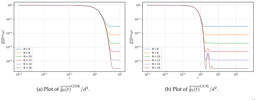
Spectral form factors of a Stabilizer Hamiltonian In this section we want to compute the remaining traces corresponding to the components of the vector ⃗ qfor a stabilizer Hamiltonian. 48 10 3 10 2 10 1 100 101 t 10 4 10 3 10 2 10 1 100 g3(t)GDE/d2 N = 6 N = 8 N = 10 N = 12 N = 14 N = 16 (a) Plot of ˜g3(t) GDE /d2. 10 3 10 2 10 1 100 101 102 t 10 4 10 3 1...
-
[23]
As the Toric code Hamiltonian is a stabilizer Hamiltonian we can exploit the results of App
Spectral form factors for the T oric Code Hamiltonian Our goal is to compute the Haar and Clifford spectral form factors for the operator VTor. As the Toric code Hamiltonian is a stabilizer Hamiltonian we can exploit the results of App. F 1 to cut the computation short. As the Toric code Hamiltonian can be exactly diagonalized, we are going to write expli...
-
[24]
This corresponds to the first delta on the rhs of (F9)
the stabilizer operators composing P (j′,k′) v′f ′ are exactly the same as the ones composing P (j,k) vf . This corresponds to the first delta on the rhs of (F9)
-
[25]
This corresponds to the second and third Kronecker delta of Eq
the stabilizer operators appearing in P (j′,k′) v′f ′ are such that all the vertex (facet) operators are the same as in P (j,k) vf , while the facet (vertex) operators in P (j′,k′) v′f ′ are exactly al the ones missing in P (j,k) vf , so that their product still gives the identity. This corresponds to the second and third Kronecker delta of Eq. (F9)
-
[26]
finally, one could have that both the vertex and facet operators appearing inP (j′,k′) v′f ′ are the ones missing in the expression ofP (j,k) vf in order to obtain the identity. This gives the fourth delta. We are now ready to compute the components of both⃗ cand ⃗ qfor the Toric code, that is, we are going to compute the regular spectral form factors gto...
-
[27]
Loschmidt echo We can write the expressions for the Loschmidt echo of the second kind in matrix notation, which are more useful for practical calculations. We have: ⟨L2(t)⟩U =⃗ cW· ⃗LH 2 (G1) ⟨L2(t)⟩C =⃗ qW+⃗LQ 2 +⃗ q⊥W −⃗LQ⊥ 2 (G2) ⟨L2(t)⟩Ck = ⃗tΞ k ⃗LQ 2 + ⃗tΓ (k) ⃗LH 2 + ⃗b· ⃗LH 2 (G3) where we have defined: (⃗LH 2 )π = Tr TπT(14)(23)A⊗2,2 (G4) (⃗LQ 2 ...
-
[28]
In particular, we assume A and B to be non-overlapping, i.e
OTOC Also in this case to compute the components of the vectors ⃗OH 4 , ⃗OQ 4 , ⃗OQ⊥ 4 one has to compute the traces of the form Tr TπA⊗1,1 ⊗B ⊗1,1 and Tr TπQA⊗1,1 ⊗B ⊗1,1 . In particular, we assume A and B to be non-overlapping, i.e. different and commuting, Pauli strings. The values of these traces are reported in Table XI. Tπ Tr TπP⊗2 ⊗P ′⊗2 Tr TπQP⊗2 ...
-
[29]
Entanglement entropy Another context in which the isospectral twirling reveals useful is the evolution of entanglement [56, 57, 116, 119, 189–195]. In fact, an important measure of the entanglement present in a quantum system is the set of α-Rényi entropies. They have found wide use in diverse field, such as condensed matter [196, 197], quantum field theo...
-
[30]
T ripartite Mutual Information Thus, in order to compute the components of the vectors ⃗I H 3,C2 , ⃗I Q 3,C2 , ⃗I Q⊥ 3,C2 needs to compute traces of the form Tr h TπT(C)⊗2 (12) i , Tr h TπT(C) (12) ⊗T (D) (12) i , Tr h TπQT(C)⊗2 (12) i , and Tr h TπQT(C) (12) ⊗T (D) (12) i , whose values are reported in Table XIII and Table XIV Let us write down the avera...
-
[31]
Coherence Quantum coherence is one of the most striking features of quantum theory, being responsible for all the observed interference phenomena. Besides its foundational role [201–204], quantum coherence is also a precious resource in quantum information processing [205–208] and thermodynamics [209–216]. Moreover, it serves as a signature of quantum cha...
-
[32]
Wigner-Yanase-Dyson Skew Information Another measure of coherence is given by the Wigner-Yanase-Dyson (WYD) skew information [228– 230]. The WYD skew information quantifies how hard it is to measure a certain observableX on a certain state ψt. In other words, it provides a measure of the strictly quantum uncertainty associated with the measurement of an o...
discussion (0)
Sign in with ORCID, Apple, or X to comment. Anyone can read and Pith papers without signing in.