Debiased Machine Learning for Conformal Prediction of Counterfactual Outcomes Under Runtime Confounding
Pith reviewed 2026-05-13 17:02 UTC · model grok-4.3
The pith
Debiased machine learning enables valid conformal prediction intervals for counterfactual outcomes when target populations have incomplete confounder data.
A machine-rendered reading of the paper's core claim, the machinery that carries it, and where it could break.
Core claim
The central claim is that a computationally efficient debiased machine learning framework, grounded in semiparametric efficiency theory, produces valid prediction intervals for counterfactual outcomes under runtime confounding, where only a subset of confounders is measured in the target population, achieving desired coverage rates with faster convergence compared to standard methods.
What carries the argument
The debiased machine learning estimator based on semiparametric efficiency theory that corrects for the bias from unmeasured confounders in the target population while enabling conformal prediction intervals.
Load-bearing premise
The debiased estimator maintains valid coverage under regularity conditions on the nuisance estimators and data distributions that hold when only a subset of confounders is observed in the target population.
What would settle it
Run synthetic experiments with known true counterfactuals and runtime confounding, then check if the empirical coverage of the prediction intervals equals the nominal level, such as 95 percent, while verifying faster convergence rates.
Figures


read the original abstract
Data-driven decision making frequently relies on predicting counterfactual outcomes. In practice, researchers commonly train counterfactual prediction models on a source dataset to inform decisions on a possibly separate target population. Conformal prediction has arisen as a popular method for producing assumption-lean prediction intervals for counterfactual outcomes that would arise under different treatment decisions in the target population of interest. However, existing methods require that every confounding factor of the treatment-outcome relationship used for training on the source data is additionally measured in the target population, risking miscoverage if important confounders are unmeasured in the target population. In this paper, we introduce a computationally efficient debiased machine learning framework that allows for valid prediction intervals when only a subset of confounders is measured in the target population, a common challenge referred to as runtime confounding. Grounded in semiparametric efficiency theory, we show the resulting prediction intervals achieve desired coverage rates with faster convergence compared to standard methods. Through numerous synthetic and semi-synthetic experiments, we demonstrate the utility of our proposed method.
Editorial analysis
A structured set of objections, weighed in public.
Referee Report
Summary. The paper introduces a computationally efficient debiased machine learning framework for conformal prediction of counterfactual outcomes under runtime confounding, where only a subset of confounders is measured in the target population. Grounded in semiparametric efficiency theory, it claims that the resulting prediction intervals achieve valid coverage with faster convergence rates than standard methods, as demonstrated in synthetic and semi-synthetic experiments.
Significance. If the central theoretical claims hold, the work is significant for practical causal inference and decision-making applications. It extends conformal prediction to settings with incomplete confounder measurements at runtime, a common real-world issue, while leveraging semiparametric efficiency to improve convergence. The provision of experiments on both synthetic and semi-synthetic data strengthens the empirical case for utility.
major comments (2)
- [§3] §3 (efficient influence function and debiased estimator): the o_p(n^{-1/2}) remainder in the semiparametric expansion is asserted to hold under runtime confounding, but the derivation does not explicitly show how the debiasing step (via projection or reweighting from source data) cancels all first-order bias terms arising from unobserved confounders in the target; without additional rate conditions on the conditional distributions of the missing confounders, the uniform validity of the expansion over the target distribution is not guaranteed.
- [§4] Theorem on coverage (likely §4): the faster convergence claim for the conformal intervals relies on the debiased estimator attaining the efficiency bound, yet the proof sketch does not address whether the quantile estimation step inherits the same remainder control when the target data lacks full confounders; this is load-bearing for the validity guarantee.
minor comments (2)
- The abstract and introduction could more explicitly list the regularity conditions (e.g., on nuisance estimator rates and positivity) required for the semiparametric results to apply.
- Notation for the source and target distributions (e.g., P_S vs. P_T) is introduced but used inconsistently in early sections; a dedicated notation table would improve clarity.
Simulated Author's Rebuttal
We thank the referee for their constructive comments, which identify areas where the theoretical derivations can be made more explicit. We address each major comment below and will incorporate the suggested clarifications in the revised manuscript.
read point-by-point responses
-
Referee: [§3] §3 (efficient influence function and debiased estimator): the o_p(n^{-1/2}) remainder in the semiparametric expansion is asserted to hold under runtime confounding, but the derivation does not explicitly show how the debiasing step (via projection or reweighting from source data) cancels all first-order bias terms arising from unobserved confounders in the target; without additional rate conditions on the conditional distributions of the missing confounders, the uniform validity of the expansion over the target distribution is not guaranteed.
Authors: We agree that the current presentation of the semiparametric expansion in §3 would benefit from greater explicitness. We will revise this section to include a step-by-step derivation demonstrating how the debiasing terms (via projection onto the observed confounders and reweighting from the source data) cancel all first-order bias contributions from the unobserved confounders. We will also state the precise rate conditions required on the conditional distributions of the missing confounders to guarantee that the o_p(n^{-1/2}) remainder holds uniformly over the target distribution. These additions will not alter the stated assumptions but will make the argument self-contained. revision: yes
-
Referee: [§4] Theorem on coverage (likely §4): the faster convergence claim for the conformal intervals relies on the debiased estimator attaining the efficiency bound, yet the proof sketch does not address whether the quantile estimation step inherits the same remainder control when the target data lacks full confounders; this is load-bearing for the validity guarantee.
Authors: We concur that the proof sketch in §4 should explicitly verify inheritance of the remainder control by the quantile estimation step. We will expand the proof to show that, because the debiased estimator attains the semiparametric efficiency bound under the runtime confounding setup, the empirical quantile of the conformal scores inherits the same o_p(n^{-1/2}) control even when the target sample observes only a subset of confounders. This will be done by bounding the difference between the estimated and oracle quantiles using the efficiency result and standard empirical process arguments that do not require full confounder observation in the target. revision: yes
Circularity Check
No circularity: claims grounded in external semiparametric efficiency theory with no self-referential reduction or fitted-input predictions.
full rationale
The paper's central contribution is a debiased machine learning framework for conformal prediction intervals under runtime confounding. It explicitly states that the method is 'Grounded in semiparametric efficiency theory' and shows coverage and faster convergence 'compared to standard methods.' No equations, influence-function expansions, or nuisance-estimator steps are shown to reduce by construction to fitted parameters or self-citations; the derivation is presented as an application of established external theory rather than a self-contained loop. The provided text contains no load-bearing self-citations, ansatzes smuggled via prior work, or renamings of known results as new derivations. This is the most common honest non-finding: the result is self-contained against external benchmarks.
Axiom & Free-Parameter Ledger
Reference graph
Works this paper leans on
-
[1]
Lettingh(Y(a),V) :=I(R a(Y,V)≤r a,α), Equation (4) immediately follows by Lemma 5
The desired result holds by recalling the definitions ofq a(ra,α,X)andm a(ra,α,V). Lettingh(Y(a),V) :=I(R a(Y,V)≤r a,α), Equation (4) immediately follows by Lemma 5. A.4. Proof of Theorem 3 SupposeO∼P, and let{P ε :ε∈[0,1)}be a generic regular parametric submodel containing the true data-generating distribution atε= 0 :P 0 =P. Recall that aninfluence curv...
work page 2006
-
[2]
ShowP(Y(a)∈ ˆCa(V)|S= 0)−(1−α) =E[χ a(O,ˆra,α;η)]/P(S= 0)
-
[3]
DecomposeE[χ a(O,ˆra,α η)]into a term whose asymptotic behavior is dominated byE(χa(ˆra,α,ˆη)− χa(ˆra,α, η)) 21 BARNATCHEZJOSEYNETHERYPARMIGIANI
-
[4]
Show that for anyr, the differenceE(χ a(r,ˆη)−χ a(r, η))satisfies the product bias structure specified in Theorem 4
-
[5]
Take the supremum of this bias structure over allrto boundE(χ a(ˆra,α,ˆη)−χ a(ˆra,α, η)) To begin, notice P(Y(a)∈ ˆCa(V)|S= 0)−(1−α) =P(R a(Y(a),V)≤ˆr a,α)|S= 0)−(1−α) =E[χ a(O,ˆra,α;η)]/P(S= 0),(10) where (10) holds since P(Ra(Y(a),V)≤r)|S= 0)−(1−α) =E[m a(r,V)−(1−α)|S= 0] =E[χ a(r, O;η a(r))]/P(S= 0), for anyr. Thus, demonstrating (9) amounts to showing...
work page 2000
-
[6]
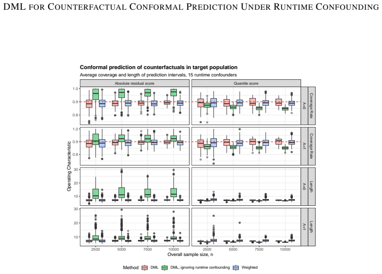
= 0.9, achieving this numerically by simulating 1 million values ofVoutside of our main simulation. Notably, source population membership is influenced byV, generating covariate shift between the source and target populations.AandY(a)are both influenced byVandU. To induce runtime confounding, we treatUas unobserved in the target population (S= 0). We setp...
work page 2020
-
[7]
Construct1−α/2level intervals ˆC1(V) = ( ˆCL 1 (V), ˆCU 1 (V))and ˆC0(V) = ( ˆCL 0 (V), ˆCU 0 (V)) forY(1)andY(0), respectively, using Algorithm 1
-
[8]
Construct intervals of the form ˆCITE(V) = ( ˆCL 1 (V)− ˆCU 0 (V), ˆCU 1 (V)− ˆCL 0 (V)) Although easy to implement, the above approach will tend to produce excessively wide intervals. Alternatively, one can construct nested intervals as outlined in Lei and Cand `es (2021) and later extended to handle target-source covariate shift in a surrogate outcome s...
work page 2021
-
[9]
Within the source population, construct intervals ˆC(X)which aim to satisfy P(Y(1)−Y(0)∈ ˆC(X)|S= 1) To do this, supposeC a(X)satisfiesP(Y(a)∈C a(X)|S= 1, A= 1−a). SinceAis observed for all units in the source population, one can construct ITE intervals in the source population of the form C(X) = ( Y−C 0(X), A·S= 1, C1(X)−Y,(1−A)·S= 1 The component interv...
work page 2024
-
[10]
Define a conformity scoreR C(C,V)with respect to the individual-level intervals ˆC(X i) in the source population. Gao et al. (2025) provide recommendations for choices of scores, where here we restrict the scores to incorporate onlyVsinceUis unobserved in the target population
work page 2025
-
[11]
Target the1−γquantile ofR C in the target population, denotedr γ which satisfies P(RC(C,V)≤r γ|S= 0) = 1−γ, noting under the earlier independence assumptions we will haver γ additionally satisfies E[P(RC(C,V)≤r γ|S= 1,V)|S= 0] = 1−γ. 32 DMLFORCOUNTERFACTUALCONFORMALPREDICTIONUNDERRUNTIMECONFOUNDING Given the above identifying functional, one can construct...
work page 2025
-
[12]
Assumption 5.a can be viewed as a weaker version of Assumption 4 that conditions on the full set of covariate information, which in tandem with Assumption 3 implies that the set of covariates Xthat are sufficient to control for treatment-outcome confounding in the source population are ad- ditionally sufficient to renderY(a)independent fromS. Relatedly, A...
discussion (0)
Sign in with ORCID, Apple, or X to comment. Anyone can read and Pith papers without signing in.