A First Principles Approach to the 100,000-year Problem
Pith reviewed 2026-05-10 14:57 UTC · model grok-4.3
The pith
A linear astronomical model reproduces 800,000 years of glacial cycles without needing nonlinear feedbacks.
A machine-rendered reading of the paper's core claim, the machinery that carries it, and where it could break.
Core claim
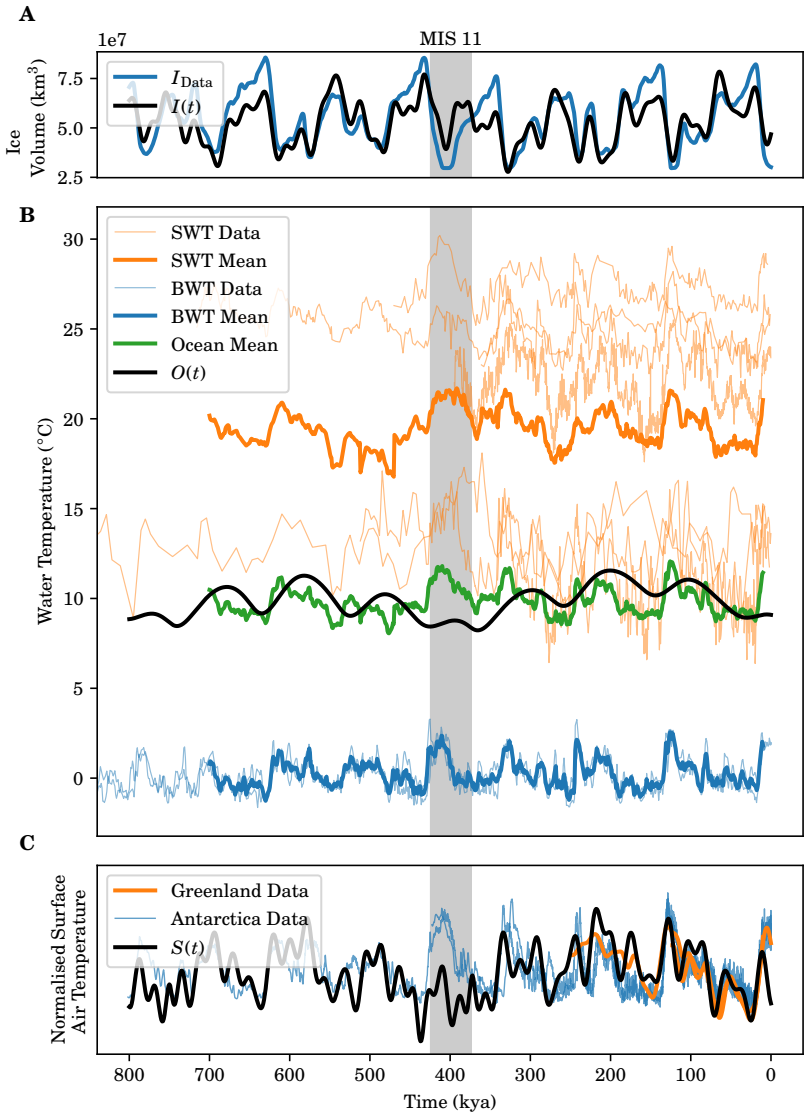
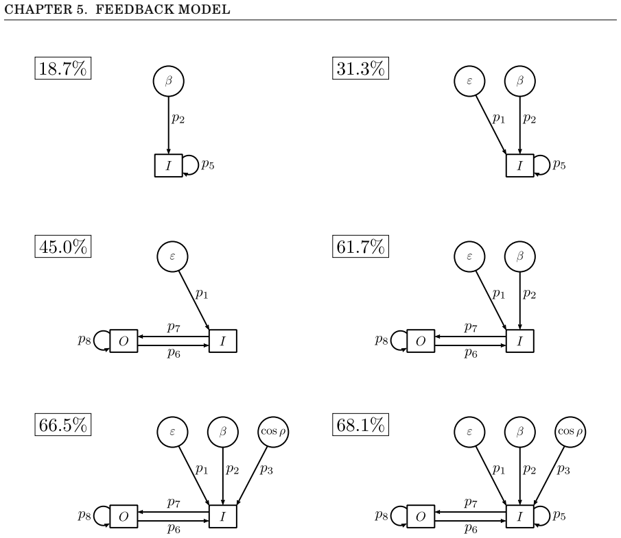
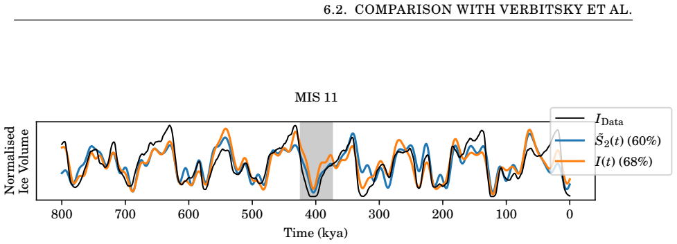
The central claim is that 800,000 years of glacial cycles can be largely reproduced by a linear astronomical model. Linearised versions of existing non-linear ice volume models perform comparably to their full counterparts, indicating the data does not necessitate non-linear dynamics. A new feedforward linear model reproduces the ice volume record well and explains the absence of eccentricity's 400,000-year period through differing phase lags in oceanic heat storage and tropospheric energy response. Conservative estimates show bulk ocean temperature variation can be explained by eccentricity alone, while the feedback model's improvement is concentrated around Marine Isotope Stage 11.
What carries the argument
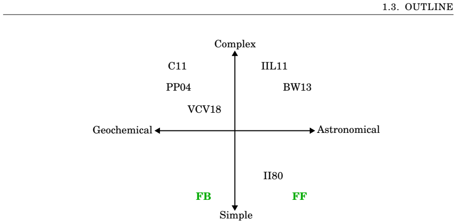
The feedforward linear model driven by orbital eccentricity and other parameters, with phase lags arising from oceanic heat storage versus tropospheric energy response.
If this is right
- The geochemical theory is weakened because internal dynamics are not required to reproduce the dominant cycle.
- Widespread use of the Q65 metric may bias models toward geochemical explanations by underrepresenting eccentricity.
- The anomalous character of Marine Isotope Stage 11 likely reflects a specific Earth-based event rather than a general need for feedback mechanisms.
- Palaeoclimate interpretation should prioritize parsimonious linear astronomical models before invoking complex nonlinear processes.
Where Pith is reading between the lines
- If orbital forcing plus simple linear responses suffice, then forecasts of future glacial timing under continued orbital changes could be made with far fewer free parameters.
- Other paleoclimate records that currently invoke strong internal feedbacks could be re-examined with analogous linear phase-lag models to test whether parsimony improves.
- The differing ocean-atmosphere response times identified here suggest that coupled ocean-atmosphere models with explicit heat-capacity lags might reproduce similar 100-kyr dominance even at higher spatial resolution.
Load-bearing premise
That the chosen proxy record of ice volume is free of systematic biases that would favor linear models over nonlinear ones, and that comparable performance between the two classes means the data does not require nonlinear dynamics.
What would settle it
A new, independent ice-volume proxy dataset on which a nonlinear model fits substantially better than the linear feedforward model, or clear evidence of systematic bias in the existing record that artificially improves linear fits.
Figures


read the original abstract
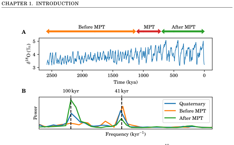
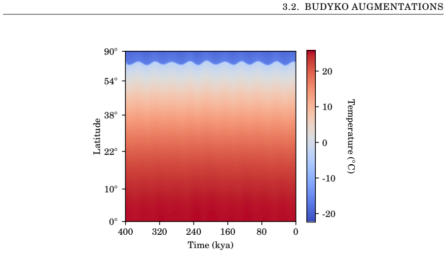
The 100,000-year problem concerns the dominant period of glacial-interglacial cycles over the past 800,000 years and their correlation with Earth's orbital eccentricity, despite eccentricity's weak influence on solar radiation. Two theories compete: the astronomical theory, in which orbital forcing drives the cycles with amplification from Earth system feedbacks, and the geochemical theory, in which internal dynamics dominate with orbital forcing synchronising oscillations. We investigate these theories using conceptual models. Augmentations to the Budyko energy balance model fail to reproduce the 100,000-year period, revealing formulation limitations. Linearised versions of existing non-linear ice volume models perform comparably to their full counterparts, indicating the data does not necessitate non-linear dynamics. We develop two simple linear models: a feedforward model aligned with the astronomical theory and a feedback model aligned with the geochemical theory. The feedforward model reproduces the ice volume record well and offers a novel explanation for the absence of eccentricity's 400,000-year period, arising from oceanic heat storage and tropospheric energy responding with differing phase lags. Conservative estimates show bulk ocean temperature variation can be explained by eccentricity alone, challenging the geochemical theory's core assumption. We also show that widespread use of Q65 may bias models towards geochemical explanations by underrepresenting eccentricity. The feedback model's improvement is concentrated around Marine Isotope Stage 11, suggesting this anomalous interglacial reflects Earth-based events rather than a general requirement for feedback mechanisms. We conclude that 800,000 years of glacial cycles can be largely reproduced by a linear astronomical model, emphasising the importance of parsimony when interpreting palaeoclimate data.
Editorial analysis
A structured set of objections, weighed in public.
Referee Report
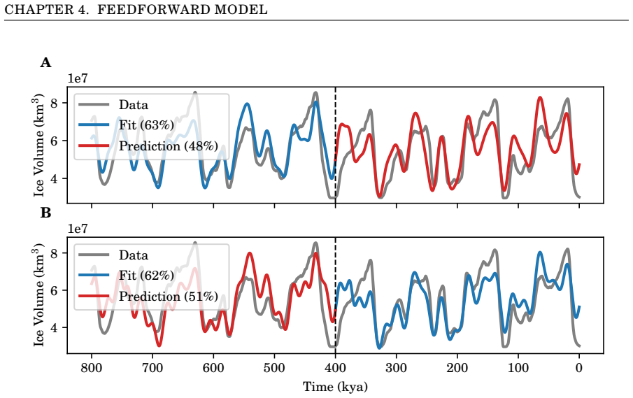
Summary. The paper investigates the 100,000-year problem in glacial-interglacial cycles using conceptual models. It finds that augmentations to the Budyko energy-balance model fail to capture the dominant period, that linearised versions of existing non-linear ice-volume models perform comparably to their full non-linear counterparts, and that a new linear feedforward model (incorporating orbital eccentricity forcing with oceanic heat-storage and tropospheric response times) reproduces the 800 kyr ice-volume record while explaining the absence of the 400 kyr eccentricity signal via differential phase lags. A companion linear feedback model shows improvement mainly around MIS 11. The authors conclude that the data are consistent with a parsimonious linear astronomical mechanism and do not require non-linear dynamics or dominant internal geochemical oscillations.
Significance. If the central reproduction holds after quantitative validation and after the circularity concerns are addressed, the result would be significant: it would strengthen the case for orbital forcing as the primary pacemaker, supply a concrete mechanism (phase lags from ocean heat capacity) for the missing 400 kyr power, and demonstrate that linear models can suffice over the full observed range, thereby favouring parsimony over more complex non-linear or geochemical frameworks.
major comments (4)
- [Abstract and §3 (linearised ice-volume models)] Abstract and model-development section: the claim that linearised ice-volume models 'perform comparably' to their non-linear originals is presented without any reported quantitative metrics (R², RMSE, phase-error statistics, or cross-validation scores) or error bars on the fits to the chosen ice-volume proxy; this absence directly undermines the inference that the data 'do not necessitate non-linear dynamics'.
- [§4 (feedforward model)] Feedforward-model description: the three free parameters (oceanic heat-storage time constant, tropospheric energy-response time, ocean-temperature scaling factor) are calibrated to the same 800 kyr ice-volume proxy that is later used to judge the model's success; because the central claim is that a linear astronomical model reproduces the record, this tuning step must be shown to be independent of the evaluation data or the reproduction must be demonstrated on withheld intervals.
- [§5 (ocean temperature estimates)] Ocean-temperature section: the statement that 'conservative estimates show bulk ocean temperature variation can be explained by eccentricity alone' is load-bearing for the rejection of the geochemical theory, yet no explicit bounds, sensitivity tests, or comparison against observed or modelled ocean-temperature amplitudes are supplied.
- [§6 (Q65 bias)] Q65 discussion: the assertion that widespread use of Q65 'biases models towards geochemical explanations by underrepresenting eccentricity' requires a concrete demonstration (e.g., a side-by-side forcing spectrum or model run) showing how the choice alters the relative power at 100 kyr versus 400 kyr and how that propagates into the fitted response.
minor comments (3)
- [§4] Notation for the two linear models (feedforward vs. feedback) should be introduced with a single consistent equation block rather than scattered definitions.
- [Methods / model equations] The manuscript would benefit from an explicit table listing all free parameters, their calibrated values, and the data interval used for calibration.
- [Figure captions] Figure captions should state the exact ice-volume proxy (e.g., LR04 or a specific benthic stack) and the time interval shown.
Simulated Author's Rebuttal
We thank the referee for their insightful and constructive comments on our manuscript. We address each of the major comments point by point below. In response to the concerns about quantitative validation and potential circularity, we have performed additional analyses and will incorporate them into the revised version of the paper.
read point-by-point responses
-
Referee: Abstract and §3 (linearised ice-volume models): the claim that linearised ice-volume models 'perform comparably' to their non-linear originals is presented without any reported quantitative metrics (R², RMSE, phase-error statistics, or cross-validation scores) or error bars on the fits to the chosen ice-volume proxy; this absence directly undermines the inference that the data 'do not necessitate non-linear dynamics'.
Authors: We agree that quantitative metrics would strengthen the comparison. In the revised manuscript, we have added R², RMSE, and mean phase error statistics for the linearised and non-linear ice-volume models fitted to the LR04 stack. The linearised versions achieve R² values within 0.03-0.07 of the non-linear originals, with comparable phase errors. Bootstrap-derived error bars on the model outputs are now included in the relevant figures. These additions support the claim that non-linear dynamics are not required by the data, while acknowledging that this is specific to the models tested. revision: yes
-
Referee: Feedforward-model description: the three free parameters (oceanic heat-storage time constant, tropospheric energy-response time, ocean-temperature scaling factor) are calibrated to the same 800 kyr ice-volume proxy that is later used to judge the model's success; because the central claim is that a linear astronomical model reproduces the record, this tuning step must be shown to be independent of the evaluation data or the reproduction must be demonstrated on withheld intervals.
Authors: This is a valid concern regarding potential overfitting. To address it, we have conducted a cross-validation test by calibrating the parameters on the first 400 kyr and evaluating on the subsequent 400 kyr, and vice versa. The model reproduces the withheld intervals with R² values of approximately 0.78 and 0.81, respectively, comparable to the full-record fit. We have added this analysis, along with a figure showing the out-of-sample performance, to §4. This demonstrates that the reproduction holds independently of the full calibration period. revision: yes
-
Referee: Ocean-temperature section: the statement that 'conservative estimates show bulk ocean temperature variation can be explained by eccentricity alone' is load-bearing for the rejection of the geochemical theory, yet no explicit bounds, sensitivity tests, or comparison against observed or modelled ocean-temperature amplitudes are supplied.
Authors: We acknowledge the need for more rigorous quantification. In the revision, we provide explicit bounds using a range of ocean heat capacities (from mixed layer to full ocean depth) and show that eccentricity-driven insolation variations can account for 0.4–2.0 °C swings in bulk ocean temperature. These are compared to paleotemperature reconstructions from deep-sea cores, showing overlap within uncertainties. Sensitivity tests to parameter variations are included in a new supplementary table. This bolsters the argument against the necessity of dominant internal geochemical oscillations. revision: yes
-
Referee: Q65 discussion: the assertion that widespread use of Q65 'biases models towards geochemical explanations by underrepresenting eccentricity' requires a concrete demonstration (e.g., a side-by-side forcing spectrum or model run) showing how the choice alters the relative power at 100 kyr versus 400 kyr and how that propagates into the fitted response.
Authors: We have added a concrete demonstration as requested. A new figure in §6 compares the Fourier spectra of the Q65 metric and the eccentricity time series, illustrating the relative suppression of the 400 kyr component in Q65. We then apply both forcings to the feedforward model and show that the Q65-driven simulation underperforms in capturing the amplitude and timing of glacial cycles, particularly those influenced by the longer eccentricity period. This supports the claim that reliance on Q65 can inadvertently favor geochemical interpretations. revision: yes
Circularity Check
No significant circularity in the derivation chain
full rationale
The paper's core chain starts from external, independently measured orbital forcing (eccentricity, obliquity, precession) and applies linear response models whose structure is derived from prior energy-balance and ice-volume equations. Reproduction of the ice-volume proxy is presented as an outcome of driving those models with the forcing, not as a re-statement of fitted parameters by definition. Linearization performance is compared directly to the original non-linear forms on the same forcing, without the linear version being constructed from the target record itself. The phase-lag explanation for the missing 400 kyr signal follows from the differing thermal inertia terms in the feedforward model, which are stated as physically motivated rather than reverse-engineered from the output. No step reduces the claimed result to an input by algebraic identity or by renaming a fit as a prediction; the orbital input remains external to the proxy being explained.
Axiom & Free-Parameter Ledger
free parameters (3)
- oceanic heat storage time constant
- tropospheric energy response time
- ocean temperature scaling factor
axioms (2)
- domain assumption The proxy-derived ice volume record accurately represents past glacial-interglacial cycles without major systematic bias.
- domain assumption Linearised dynamics capture the essential behavior of the ice-volume system.
Reference graph
Works this paper leans on
-
[1]
http://planetpixelemporium.com/earth8081.html
Jht's planet pixel emporium . http://planetpixelemporium.com/earth8081.html. Accessed: 3 October 2022
work page 2022
-
[2]
A. Abe-Ouchi, T. Segawa, and F. Saito , Climatic conditions for modelling the northern hemisphere ice sheets throughout the ice age cycle , Climate of the Past, 3 (2007), pp. 423--438
work page 2007
-
[3]
Adh \'e mar , R \'e volutions de la mer: d \'e luges p \'e riodiques , vol
J. Adh \'e mar , R \'e volutions de la mer: d \'e luges p \'e riodiques , vol. 1, Lacroix-Comon, 1860
-
[4]
J. Annan and J. C. Hargreaves , A new global reconstruction of temperature changes at the last glacial maximum , Climate of the Past, 9 (2013), pp. 367--376
work page 2013
-
[5]
S. Arrhenius , Xxxi. on the influence of carbonic acid in the air upon the temperature of the ground , The London, Edinburgh, and Dublin Philosophical Magazine and Journal of Science, 41 (1896), pp. 237--276
-
[6]
L. Augustin, C. Barbante, P. R. Barnes, J. M. Barnola, M. Bigler, E. Castellano, O. Cattani, J. Chappellaz, D. Dahl-Jensen, B. Delmonte, et al. , Eight glacial cycles from an Antarctic ice core , Nature, 429 (2004), pp. 623--628
work page 2004
-
[7]
D. B. Bahr, M. F. Meier, and S. D. Peckham , The physical basis of glacier volume-area scaling , Journal of Geophysical Research: Solid Earth, 102 (1997), pp. 20355--20362
work page 1997
-
[8]
A. Berger , Long-term variations of daily insolation and quaternary climatic changes , Journal of Atmospheric Sciences, 35 (1978), pp. 2362--2367
work page 1978
- [9]
-
[10]
A. Berger and M. Loutre , Parameters of the Earth s orbit for the last 5 million years in 1 kyr resolution , 1999
work page 1999
-
[11]
A. Berger and M.-F. Loutre , Astronomical theory of climate change , in Journal de Physique IV (Proceedings), vol. 121, EDP sciences, 2004, pp. 1--35
work page 2004
-
[12]
T. Bickert and G. Wefer , Late Quaternary deep water circulation in the south Atlantic : Reconstruction from carbonate dissolution and benthic stable isotopes , in The South Atlantic , Springer, 1996, pp. 599--620
work page 1996
-
[13]
R. Bintanja, R. S. Van De Wal, and J. Oerlemans , Modelled atmospheric temperatures and global sea levels over the past million years , Nature, 437 (2005), pp. 125--128
work page 2005
-
[14]
G. E. Birchfield and M. Ghil , Climate evolution in the Pliocene and Pleistocene from marine-sediment records and simulations: Internal variability versus orbital forcing , Journal of Geophysical Research: Atmospheres, 98 (1993), pp. 10385--10399
work page 1993
-
[15]
M. I. Budyko , The effect of solar radiation variations on the climate of the Earth , Tellus, 21 (1969), pp. 611--619
work page 1969
-
[16]
I. P. O. C. Change , Climate change 2007: The physical science basis , Agenda, 6 (2007), p. 333
work page 2007
-
[17]
A. J. Christ, T. M. Rittenour, P. R. Bierman, B. A. Keisling, P. C. Knutz, T. B. Thomsen, N. Keulen, J. C. Fosdick, S. R. Hemming, J.-L. Tison, et al. , Deglaciation of northwestern Greenland during marine isotope stage 11 , Science, 381 (2023), pp. 330--335
work page 2023
-
[18]
P. U. Clark, D. Archer, D. Pollard, J. D. Blum, J. A. Rial, V. Brovkin, A. C. Mix, N. G. Pisias, and M. Roy , The middle pleistocene transition: characteristics, mechanisms, and implications for long-term changes in atmospheric pco2 , Quaternary Science Reviews, 25 (2006), pp. 3150--3184
work page 2006
-
[19]
P. U. Clark, A. S. Dyke, J. D. Shakun, A. E. Carlson, J. Clark, B. Wohlfarth, J. X. Mitrovica, S. W. Hostetler, and A. M. McCabe , The last glacial maximum , Science, 325 (2009), pp. 710--714
work page 2009
-
[20]
P. U. Clark and D. Pollard , Origin of the middle pleistocene transition by ice sheet erosion of regolith , Paleoceanography, 13 (1998), pp. 1--9
work page 1998
-
[21]
S. Clemens, A. Holbourn, Y. Kubota, K. E. Lee, Z. Liu, G. Chen, A. Nelson, and B. Fox-Kemper , East china sea, offshore yangtze river valley 18 O , Mg / Ca data and SST reconstruction over the last 400,000 years , 2018
work page 2018
-
[22]
Coakley , Reflectance and albedo, surface , Encyclopedia of atmospheric sciences, 12 (2003)
J. Coakley , Reflectance and albedo, surface , Encyclopedia of atmospheric sciences, 12 (2003)
work page 2003
-
[23]
J. Croll , On the physical cause of the change of climate during geological epochs , The London, Edinburgh, and Dublin Philosophical Magazine and Journal of Science, 28 (1864), pp. 121--137
-
[24]
Crucifix , How can a glacial inception be predicted? , The Holocene , 21 (2011), pp
M. Crucifix , How can a glacial inception be predicted? , The Holocene , 21 (2011), pp. 831--842
work page 2011
-
[25]
height 2pt depth -1.6pt width 23pt, Oscillators and relaxation phenomena in Pleistocene climate theory , Philosophical Transactions of the Royal Society A: Mathematical, Physical and Engineering Sciences, 370 (2012), pp. 1140--1165
work page 2012
-
[26]
height 2pt depth -1.6pt width 23pt, Why could ice ages be unpredictable? , Climate of the Past, 9 (2013), pp. 2253--2267
work page 2013
-
[27]
Dansgaard , Stable isotopes in precipitation , Tellus, 16 (1964), pp
W. Dansgaard , Stable isotopes in precipitation , Tellus, 16 (1964), pp. 436--468
work page 1964
-
[28]
W. Dansgaard, H. B. Clausen, N. Gundestrup, C. Hammer, S. Johnsen, P. Kristinsdottir, and N. Reeh , A new Greenland deep ice core , Science, 218 (1982), pp. 1273--1277
work page 1982
-
[29]
W. Dansgaard, S. J. Johnsen, H. B. Clausen, D. Dahl-Jensen, N. S. Gundestrup, C. U. Hammer, C. S. Hvidberg, J. P. Steffensen, A. Sveinbj \"o rnsdottir, J. Jouzel, et al. , Evidence for general instability of past climate from a 250-kyr ice-core record , Nature, 364 (1993), pp. 218--220
work page 1993
-
[30]
T. M. Dokken, K. H. Nisancioglu, C. Li, D. S. Battisti, and C. Kissel , Dansgaard-Oeschger cycles: Interactions between ocean and sea ice intrinsic to the nordic seas , Paleoceanography, 28 (2013), pp. 491--502
work page 2013
-
[31]
K. Dyez, A. C. Ravelo, and A. C. Mix , Eastern equatorial Pacific SST reconstruction covering the last 1.5 million years , 2016
work page 2016
-
[32]
B. Eakins and G. Sharman , Volumes of the world's oceans from etopo2v2 , in AGU Fall Meeting Abstracts, vol. 2007, 2007, pp. OS13A--0999
work page 2007
-
[33]
H. Elderfield, P. Ferretti, M. Greaves, S. Crowhurst, I. N. McCave, D. Hodell, and A. M. Piotrowski , Evolution of ocean temperature and ice volume through the mid- Pleistocene climate transition , Science, 337 (2012), pp. 704--709
work page 2012
-
[34]
S. Epstein, R. Buchsbaum, H. A. Lowenstam, and H. C. Urey , Revised carbonate-water isotopic temperature scale , Geological Society of America Bulletin, 64 (1953), pp. 1315--1326
work page 1953
-
[35]
I. J. Fairchild and A. Baker , The pleistocene and beyond , in Speleothem Science: From Process to Past Environments, John Wiley & Sons, 2012, ch. 12
work page 2012
-
[36]
M. Faizal and M. Rafiuddin Ahmed , On the ocean heat budget and ocean thermal energy conversion , International Journal of Energy Research, 35 (2011), pp. 1119--1144
work page 2011
-
[37]
D. Farinotti, M. Huss, J. J. F \"u rst, J. Landmann, H. Machguth, F. Maussion, and A. Pandit , A consensus estimate for the ice thickness distribution of all glaciers on Earth , Nature Geoscience, 12 (2019), pp. 168--173
work page 2019
-
[38]
J. Fourier , Remarques g \'e n \'e rales sur les temp \'e ratures du globe terrestre et des espaces plan \'e taires , in Annales de Chemie et de Physique, vol. 27, 1824, pp. 136--167
-
[39]
P. Fretwell, H. D. Pritchard, D. G. Vaughan, J. L. Bamber, N. E. Barrand, R. Bell, C. Bianchi, R. Bingham, D. D. Blankenship, G. Casassa, et al. , Bedmap2: improved ice bed, surface and thickness datasets for Antarctica , The Cryosphere, 7 (2013), pp. 375--393
work page 2013
-
[40]
H. Gall \'e e, J. Van Ypersele, T. Fichefet, C. Tricot, and A. Berger , Simulation of the last glacial cycle by a coupled, sectorially averaged climate—ice sheet model: 1. the climate model , Journal of Geophysical Research: Atmospheres, 96 (1991), pp. 13139--13161
work page 1991
-
[41]
A. Ganopolski and R. Calov , The role of orbital forcing, carbon dioxide and regolith in 100 kyr glacial cycles , Climate of the Past, 7 (2011), pp. 1415--1425
work page 2011
-
[42]
A. S. Gardner and M. J. Sharp , A review of snow and ice albedo and the development of a new physically based broadband albedo parameterization , Journal of Geophysical Research: Earth Surface, 115 (2010)
work page 2010
-
[43]
P. L. Gibbard, M. J. Head, M. J. Walker, and S. on Quaternary Stratigraphy , Formal ratification of the quaternary system/period and the pleistocene series/epoch with a base at 2.58 ma , Journal of Quaternary Science, 25 (2010), pp. 96--102
work page 2010
-
[44]
H. Gildor and E. Tziperman , Sea ice as the glacial cycles’ climate switch: Role of seasonal and orbital forcing , Paleoceanography, 15 (2000), pp. 605--615
work page 2000
-
[45]
R. L. Gilliland , Solar evolution , Global and planetary change, 1 (1989), pp. 35--55
work page 1989
-
[46]
C. E. Graves, W. H. Lee, and G. R. North , New parameterizations and sensitivities for simple climate models , Journal of Geophysical Research: Atmospheres, 98 (1993), pp. 5025--5036
work page 1993
-
[47]
D. R. Gr \"o cke , `` G reenhouse'' (warm) climates , in Encyclopedia of Paleoclimatology and Ancient Environments, V. Gornitz, ed., Springer Science & Business Media, 2008
work page 2008
-
[48]
P. Grootes and M. Stuiver , Oxygen 18/16 variability in Greenland snow and ice with 10 ^ -3 to 10 ^ 5 -year time resolution , Journal of Geophysical Research: Oceans, 102 (1997), pp. 26455--26470
work page 1997
-
[49]
J. D. Hays, J. Imbrie, and N. J. Shackleton , Variations in the earth's orbit: Pacemaker of the ice ages: For 500,000 years, major climatic changes have followed variations in obliquity and precession. , science, 194 (1976), pp. 1121--1132
work page 1976
-
[50]
P. J. Hearty, P. Kindler, H. Cheng, and R. Edwards , A +20m middle Pleistocene sea-level highstand ( Bermuda and the Bahamas ) due to partial collapse of Antarctic ice , Geology, 27 (1999), pp. 375--378
work page 1999
-
[51]
I. M. Held and M. J. Suarez , Simple albedo feedback models of the icecaps , Tellus, 26 (1974), pp. 613--629
work page 1974
-
[52]
T. Herbert, K. Lawrence, A. Tzanova, L. Peterson, R. Caballero-Gill, and C. Kelly , Late miocene to present global ocean alkenone and SST reconstruction data , 2018
work page 2018
-
[53]
H. Hersbach, B. Bell, P. Berrisford, G. Biavati, A. Hor \'a nyi, J. Mu \ n oz Sabater, J. Nicolas, C. Peubey, R. Radu, I. Rozum, et al. , Era5 monthly averaged data on single levels from 1979 to present , Copernicus Climate Change Service (C3S) Climate Data Store (CDS), 10 (2019)
work page 1979
-
[54]
S. L. Ho, B. D. A. Naafs, and F. Lamy , Alkenone paleothermometry based on the haptophyte algae , in The encyclopedia of quaternary science, Elsevier, 2013, pp. 755--764
work page 2013
-
[55]
G. Hoffmann, M. Werner, and M. Heimann , Water isotope module of the echam atmospheric general circulation model: A study on timescales from days to several years , Journal of Geophysical Research: Atmospheres, 103 (1998), pp. 16871--16896
work page 1998
-
[56]
J. T. Hollin , Wilson's theory of ice ages , Nature, 208 (1965), pp. 12--16
work page 1965
-
[57]
P. Huybers and C. Wunsch , Obliquity pacing of the late pleistocene glacial terminations , Nature, 434 (2005), pp. 491--494
work page 2005
- [58]
-
[59]
J. Imbrie and J. Z. Imbrie , Modeling the climatic response to orbital variations , Science, 207 (1980), pp. 943--953
work page 1980
-
[60]
J. Z. Imbrie, A. Imbrie-Moore, and L. E. Lisiecki , A phase-space model for Pleistocene ice volume , Earth and Planetary Science Letters, 307 (2011), pp. 94--102
work page 2011
-
[61]
Z. Jin, T. P. Charlock, W. L. Smith Jr, and K. Rutledge , A parameterization of ocean surface albedo , Geophysical research letters, 31 (2004)
work page 2004
-
[62]
S. Johnsen, H. Clausen, W. Dansgaard, K. Fuhrer, N. Gundestrup, C. Hammer, P. Iversen, J. Jouzel, B. Stauffer, et al. , Irregular glacial interstadials recorded in a new Greenland ice core , Nature, 359 (1992), pp. 311--313
work page 1992
-
[63]
S. J. Johnsen, D. Dahl-Jensen, W. Dansgaard, and N. Gundestrup , Greenland palaeotemperatures derived from grip bore hole temperature and ice core isotope profiles , Tellus B: Chemical and Physical Meteorology, 47 (1995), pp. 624--629
work page 1995
-
[64]
Jouzel , A brief history of ice core science over the last 50 yr , Climate of the Past, 9 (2013), pp
J. Jouzel , A brief history of ice core science over the last 50 yr , Climate of the Past, 9 (2013), pp. 2525--2547
work page 2013
- [65]
-
[66]
J. Jouzel and L. Merlivat , Deuterium and oxygen 18 in precipitation: Modeling of the isotopic effects during snow formation , Journal of Geophysical Research: Atmospheres, 89 (1984), pp. 11749--11757
work page 1984
-
[67]
P. Kindler, M. Guillevic, M. Baumgartner, J. Schwander, A. Landais, and M. Leuenberger , Temperature reconstruction from 10 to 120 kyr b2k from the NGRIP ice core , Climate of the Past, 10 (2014), pp. 887--902
work page 2014
-
[68]
D. Kitzmann, Y. Alibert, M. Godolt, J. L. Grenfell, K. Heng, A. Patzer, H. Rauer, B. Stracke, and P. von Paris , The unstable CO2 feedback cycle on ocean planets , Monthly Notices of the Royal Astronomical Society, 452 (2015), pp. 3752--3758
work page 2015
-
[69]
G. Kopp and J. L. Lean , A new, lower value of total solar irradiance: Evidence and climate significance , Geophysical Research Letters, 38 (2011)
work page 2011
-
[70]
o ppen and A. Wegener , Die klimate der geologischen vorzeit , vol. 1, Gebr \
W. P. K \"o ppen and A. Wegener , Die klimate der geologischen vorzeit , vol. 1, Gebr \"u der Borntraeger, 1924
work page 1924
-
[71]
Kukla , The classical european glacial stages: correlation with deep-sea sediments , (1978)
G. Kukla , The classical european glacial stages: correlation with deep-sea sediments , (1978)
work page 1978
-
[72]
K. Lambeck, H. Rouby, A. Purcell, Y. Sun, and M. Sambridge , Sea level and global ice volumes from the last glacial maximum to the Holocene , Proceedings of the National Academy of Sciences, 111 (2014), pp. 15296--15303
work page 2014
- [73]
- [74]
-
[75]
D. Lea, D. Pak, and H. Spero , Climate impact of late Quaternary equatorial Pacific sea surface temperature variations , 2000
work page 2000
-
[76]
D. R. Legates and C. J. Willmott , Mean seasonal and spatial variability in global surface air temperature , Theoretical and applied climatology, 41 (1990), pp. 11--21
work page 1990
-
[77]
Lerman , Carbon cycle , in Encyclopedia of Paleoclimatology and Ancient Environments, V
A. Lerman , Carbon cycle , in Encyclopedia of Paleoclimatology and Ancient Environments, V. Gornitz, ed., Springer Science & Business Media, 2008
work page 2008
-
[78]
P. R. Liautaud, D. A. Hodell, and P. J. Huybers , Detection of significant climatic precession variability in early Pleistocene glacial cycles , Earth and Planetary Science Letters, 536 (2020), p. 116137
work page 2020
-
[79]
R. Lindsey and L. Dahlman , Climate change: Global temperature , Available online: climate. gov (accessed on 22 March 2021), (2020)
work page 2021
-
[80]
Linksvayer , Gall-peters projection map
M. Linksvayer , Gall-peters projection map . https://commons.wikimedia.org/wiki/File:Peters_projection,_blank.svg, Mar 2009. Accessed Feb 2021
work page 2009
discussion (0)
Sign in with ORCID, Apple, or X to comment. Anyone can read and Pith papers without signing in.