Recognition: unknown
From Clumps to Sheets: Geometry Controls the Temperature PDF of Multi-Phase Gas
Pith reviewed 2026-05-10 15:08 UTC · model grok-4.3
The pith
The temperature PDF of multi-phase gas is set by the geometry of isosurfaces, which transition from clumps to sheets in turbulent media.
A machine-rendered reading of the paper's core claim, the machinery that carries it, and where it could break.
Core claim
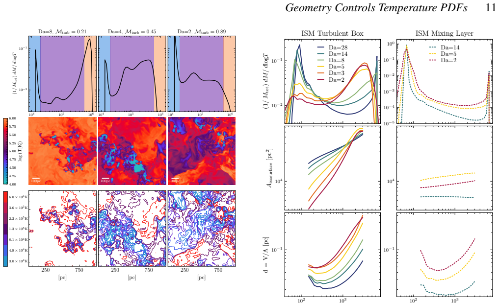
The temperature PDF can be decomposed into the product of the area of temperature isosurfaces and the thickness of the corresponding temperature layers. The thickness is controlled primarily by microphysics such as radiative cooling and thermal conduction, and is well captured by existing mixing-layer models. The isosurface area, however, is set by morphology: in mixing layers it remains sheet-like, whereas in turbulent media cold gas forms clumps whose interfaces expand with temperature and eventually percolate into connected sheets, producing broad PDFs with large intermediate-temperature mass fractions.
What carries the argument
Decomposition of the temperature PDF as the product of isosurface area and layer thickness, where morphology determines the area via clump-to-sheet transitions.
If this is right
- Broad PDFs with substantial intermediate-temperature gas arise naturally from the clump-to-sheet transition in turbulent ISM conditions.
- Thermally unstable gas fractions in the ISM are a geometric consequence rather than a microphysical one.
- The large OVI reservoir observed in the CGM is consistent with persistent sheet-like mixing layers.
- X-ray to H-alpha correlations in jellyfish galaxy tails can be interpreted through the same geometric control of temperature structure.
Where Pith is reading between the lines
- The same clump-to-sheet mechanism may govern temperature distributions in other multi-phase environments such as supernova-driven bubbles or galactic winds.
- Morphology diagnostics from emission maps could be used to predict the width of unobserved temperature PDFs in real systems.
- Varying the driving scale of turbulence in simulations would test whether the percolation threshold for sheet formation depends on the energy injection scale.
Load-bearing premise
The 3D hydrodynamic simulations under identical microphysical conditions accurately isolate geometry as the sole differing factor between ISM and CGM regimes.
What would settle it
A controlled simulation that enforces sheet-like morphology in a turbulent box yet still produces a broad temperature PDF, or an observation of temperature PDFs in a known clumpy ISM region that match the narrow widths of mixing-layer models.
Figures


read the original abstract
Temperature probability distribution functions (PDFs) are a compact description of the thermal structure of multi-phase turbulent gas, and are directly linked to observables such as emission/absorption line ratios and phase mass fractions. In the circumgalactic medium (CGM) literature, temperature PDFs are often interpreted using planar turbulent radiative mixing layers, for which analytic models successfully reproduce the simulated temperature structure. These PDFs are assumed to be universal. By contrast, studies of the multiphase interstellar medium (ISM) typically use turbulent-box simulations, which produce broad PDFs but lack a clear theoretical interpretation. Using 3D hydrodynamic simulations under both ISM and CGM conditions, we compare planar mixing layers with turbulent-box simulations under identical microphysical conditions. Despite identical cooling and turbulent driving, the resulting temperature PDFs differ substantially. The missing ingredient is geometry. We demonstrate that the temperature PDF can be decomposed into the product of the area of temperature isosurfaces and the thickness of the corresponding temperature layers. The thickness is controlled primarily by microphysics, such as radiative cooling and thermal conduction, and is well captured by existing mixing-layer models. The isosurface area, however, is set by morphology. In mixing layers it remains sheet-like, whereas in turbulent media cold gas forms clumps whose interfaces expand with temperature and eventually percolate into connected sheets. This geometric transition produces broad PDFs with large intermediate-temperature mass fractions. These results have implications for long-standing puzzles such as thermally unstable gas in the ISM, the large OVI reservoir in the CGM, and X-ray-H$\alpha$ correlations in jellyfish tails.
Editorial analysis
A structured set of objections, weighed in public.
Referee Report
Summary. The manuscript uses comparative 3D hydrodynamic simulations of planar turbulent radiative mixing layers and turbulent-box setups under identical microphysical conditions (cooling functions, conduction, turbulent driving) for ISM and CGM regimes. It claims that temperature PDFs differ substantially due to geometry: the PDF decomposes as the product of temperature-isosurface area A(T), controlled by morphology (persistent sheets in mixing layers vs. clump formation and percolation into sheets in turbulent media), and layer thickness δ(T), controlled by microphysics and matching existing planar mixing-layer models. This geometric transition is argued to produce broader PDFs with larger intermediate-temperature mass fractions in turbulent media.
Significance. If the decomposition and the insensitivity of δ(T) to global geometry hold, the work supplies a concrete physical mechanism linking morphology to observable temperature structure in multi-phase gas. It bridges analytic mixing-layer models with full turbulent simulations and offers a route to interpreting long-standing issues such as the mass fraction of thermally unstable gas in the ISM and the large OVI column in the CGM. The use of identical microphysics across setups is a clear strength that isolates geometry as the differing factor.
major comments (2)
- [§4.2] §4.2 (PDF decomposition): the central claim that δ(T) is set solely by microphysics and is insensitive to morphology requires a direct, quantitative extraction and comparison of δ(T) profiles (or equivalent local temperature gradients) from both the planar mixing-layer and turbulent-box runs; without tabulated or plotted agreement to within numerical uncertainties across the relevant temperature range, the attribution of all PDF differences to A(T) alone is not yet load-bearing.
- [§3] §3 (simulation setup and turbulent-box results): cold gas is described as forming clumps with curved interfaces that later percolate; the manuscript does not demonstrate that the effective mixing length or local temperature gradient around these curved surfaces remains identical to the planar case, leaving open the possibility that 3D straining or curvature couples back into δ(T) and undermines the clean separation from A(T).
minor comments (2)
- [Abstract] Abstract: inclusion of at least one quantitative metric (e.g., the factor by which the intermediate-temperature mass fraction differs between the two geometries, or the temperature range over which the decomposition holds) would make the strength of the result immediately clear to readers.
- Figure captions (throughout): specify the exact temperature binning and any resolution or convergence information used when computing isosurface areas and layer thicknesses.
Simulated Author's Rebuttal
We thank the referee for the constructive report and positive assessment of the work's significance. The comments identify key points where additional evidence will strengthen the central claims. We address each major comment below and will revise the manuscript to incorporate the requested comparisons.
read point-by-point responses
-
Referee: [§4.2] §4.2 (PDF decomposition): the central claim that δ(T) is set solely by microphysics and is insensitive to morphology requires a direct, quantitative extraction and comparison of δ(T) profiles (or equivalent local temperature gradients) from both the planar mixing-layer and turbulent-box runs; without tabulated or plotted agreement to within numerical uncertainties across the relevant temperature range, the attribution of all PDF differences to A(T) alone is not yet load-bearing.
Authors: We agree that the decomposition claim requires explicit quantitative support. The manuscript currently infers the insensitivity of δ(T) from the fact that the PDF differences are fully accounted for by variations in A(T), but this is indirect. In the revised version we will add a new panel (or figure) in §4.2 that extracts δ(T) (or equivalently the local |∇T|) from both the planar mixing-layer and turbulent-box runs under identical microphysics and shows agreement to within numerical uncertainties across the temperature range of interest. This will make the separation between A(T) and δ(T) load-bearing. revision: yes
-
Referee: [§3] §3 (simulation setup and turbulent-box results): cold gas is described as forming clumps with curved interfaces that later percolate; the manuscript does not demonstrate that the effective mixing length or local temperature gradient around these curved surfaces remains identical to the planar case, leaving open the possibility that 3D straining or curvature couples back into δ(T) and undermines the clean separation from A(T).
Authors: We acknowledge that the present text does not contain a direct side-by-side comparison of local temperature gradients or effective mixing lengths at curved interfaces. While the global decomposition already implies that any such effects are subdominant (otherwise the PDF would not be reproduced by A(T) alone), we will add in the revised §3 an explicit measurement of local |∇T| and mixing-layer thickness sampled around both planar and curved interfaces in the turbulent-box runs. These will be compared quantitatively to the planar mixing-layer results to confirm that curvature and straining do not materially alter δ(T). revision: yes
Circularity Check
No significant circularity; central claim from direct simulation comparisons
full rationale
The paper derives its key result—that the temperature PDF decomposes as the product of temperature-isosurface area (morphology-controlled) and layer thickness (microphysics-controlled)—from side-by-side 3D hydrodynamic simulations of planar mixing layers versus turbulent boxes run under identical cooling functions and driving. This is an empirical decomposition extracted from the numerical data rather than a self-referential definition, a fitted parameter renamed as a prediction, or a load-bearing self-citation chain. No equations or claims in the provided text reduce the target PDF back to its own inputs by construction; the geometric interpretation follows from observed morphology differences in the runs.
Axiom & Free-Parameter Ledger
axioms (2)
- standard math Hydrodynamic equations plus radiative cooling govern the evolution of multi-phase gas
- domain assumption Layer thickness is set by microphysical cooling and conduction rates
Reference graph
Works this paper leans on
-
[1]
Abruzzo M. W., Bryan G. L., Fielding D. B., 2022, @doi [ ] 10.3847/1538-4357/ac3c48 , https://ui.adsabs.harvard.edu/abs/2022ApJ...925..199A 925, 199
-
[2]
Armstrong J. W., Rickett B. J., Spangler S. R., 1995, @doi [ ] 10.1086/175515 , http://adsabs.harvard.edu/abs/1995ApJ...443..209A 443, 209
-
[3]
Audit E., Hennebelle P., 2005, @doi [ ] 10.1051/0004-6361:20041474 , http://adsabs.harvard.edu/abs/2005A
-
[4]
Beattie J. R., Kolborg A. N., Ramirez-Ruiz E., Federrath C., 2025, @doi [The Astrophysical Journal] 10.3847/1538-4357/ae07cd , 994, 193
-
[5]
C., Fabian A
Begelman M. C., Fabian A. C., 1990, , http://adsabs.harvard.edu/abs/1990MNRAS.244P..26B 244, 26P
1990
-
[6]
Cecil G., Bland-Hawthorn J., Veilleux S., 2002, @doi [ ] 10.1086/341861 , https://ui.adsabs.harvard.edu/abs/2002ApJ...576..745C 576, 745
-
[7]
Chen Z., Oh S. P., 2024, @doi [Monthly Notices of the Royal Astronomical Society] 10.1093/mnras/stae1113 , 530, 4032
-
[8]
Chen Z., Fielding D. B., Bryan G. L., 2023, @doi [ ] 10.3847/1538-4357/acc73f , https://ui.adsabs.harvard.edu/abs/2023ApJ...950...91C 950, 91
-
[9]
Modeling Emission-Line Surface Brightness in a Multiphase Galactic Wind: An O VI Case Study
Chen Z., et al., 2025, @doi [arXiv e-prints] 10.48550/arXiv.2510.02443 , https://ui.adsabs.harvard.edu/abs/2025arXiv251002443C p. arXiv:2510.02443
work page internal anchor Pith review Pith/arXiv arXiv doi:10.48550/arxiv.2510.02443 2025
-
[10]
Connor I., Beattie J. R., Kolborg A. N., Ramirez-Ruiz E., 2026, @doi [The Astrophysical Journal] 10.3847/1538-4357/ae17b1 , 997, 33
-
[11]
P., 2005, @doi [ ] 10.1146/annurev.astro.43.072103.150615 , http://adsabs.harvard.edu/abs/2005ARA
Cox D. P., 2005, @doi [ ] 10.1146/annurev.astro.43.072103.150615 , http://adsabs.harvard.edu/abs/2005ARA
-
[12]
o hler G., 1940, Zeitschrift f \
Damk \"o hler G., 1940, Zeitschrift f \"u r Elektrochemie und angewandte physikalische Chemie, 46, 601
1940
-
[13]
Das H. K., Gronke M., 2023, @doi [ ] 10.1093/mnras/stad3125 , https://ui.adsabs.harvard.edu/abs/2023MNRAS.tmp.2982D
-
[14]
Donahue M., Mack J., Voit G. M., Sparks W., Elston R., Maloney P. R., 2000, @doi [ ] 10.1086/317836 , https://ui.adsabs.harvard.edu/abs/2000ApJ...545..670D 545, 670
-
[15]
T., 2011, Physics of the Interstellar and Intergalactic Medium
Draine B. T., 2011, Physics of the Interstellar and Intergalactic Medium . Princeton University Press
2011
-
[16]
Elmegreen B. G., Scalo J., 2004, @doi [ ] 10.1146/annurev.astro.41.011802.094859 , http://adsabs.harvard.edu/abs/2004ARA
-
[17]
C., 2025, Measure theory and fine properties of functions
Evans L. C., 2025, Measure theory and fine properties of functions. Chapman and Hall/CRC
2025
-
[18]
Farber R. J., Gronke M., 2022, @doi [ ] 10.1093/mnras/stab3412 , https://ui.adsabs.harvard.edu/abs/2022MNRAS.510..551F 510, 551
-
[19]
Faucher-Gigu \`e re C.-A., Oh S. P., 2023, @doi [ ] 10.1146/annurev-astro-052920-125203 , https://ui.adsabs.harvard.edu/abs/2023ARA&A..61..131F 61, 131
-
[20]
Fielding D. B., Ostriker E. C., Bryan G. L., Jermyn A. S., 2020, @doi [ ] 10.3847/2041-8213/ab8d2c , https://ui.adsabs.harvard.edu/abs/2020ApJ...894L..24F 894, L24
-
[21]
Gaensler B. M., et al., 2011, @doi [ ] 10.1038/nature10446 , https://ui.adsabs.harvard.edu/abs/2011Natur.478..214G 478, 214
-
[22]
Gnat O., Sternberg A., 2007, @doi [ ] 10.1086/509786 , http://adsabs.harvard.edu/abs/2007ApJS..168..213G 168, 213
-
[23]
P., 2018, @doi [ ] 10.1093/mnrasl/sly131 , http://adsabs.harvard.edu/abs/2018MNRAS.tmpL.135G
Gronke M., Oh S. P., 2018, @doi [ ] 10.1093/mnrasl/sly131 , http://adsabs.harvard.edu/abs/2018MNRAS.tmpL.135G
-
[24]
Gronke M., Oh S. P., 2020a, @doi [ ] 10.1093/mnras/stz3332 , https://ui.adsabs.harvard.edu/abs/2020MNRAS.492.1970G 492, 1970
-
[25]
Gronke M., Oh S. P., 2020b, @doi [ ] 10.1093/mnrasl/slaa033 , https://ui.adsabs.harvard.edu/abs/2020MNRAS.494L..27G 494, L27
-
[26]
Gronke M., Oh S. P., Ji S., Norman C., 2022, @doi [ ] 10.1093/mnras/stab3351 , https://ui.adsabs.harvard.edu/abs/2022MNRAS.511..859G 511, 859
-
[27]
Haud U., Kalberla P. M. W., 2007, @doi [ ] 10.1051/0004-6361:20065796 , https://ui.adsabs.harvard.edu/abs/2007A&A...466..555H 466, 555
-
[28]
H., 2003, @doi [ ] 10.1086/367828 , https://ui.adsabs.harvard.edu/abs/2003ApJ...586.1067H 586, 1067
Heiles C., Troland T. H., 2003, @doi [ ] 10.1086/367828 , https://ui.adsabs.harvard.edu/abs/2003ApJ...586.1067H 586, 1067
-
[29]
Jennings R. M., Li Y., 2021, @doi [ ] 10.1093/mnras/stab1607 , https://ui.adsabs.harvard.edu/abs/2021MNRAS.505.5238J 505, 5238
-
[30]
Ji S., Oh S. P., Masterson P., 2019, @doi [ ] 10.1093/mnras/stz1248 , https://ui.adsabs.harvard.edu/abs/2019MNRAS.487..737J 487, 737
-
[31]
Jiang Y.-F., Oh S. P., 2018, @doi [ ] 10.3847/1538-4357/aaa6ce , http://adsabs.harvard.edu/abs/2018ApJ...854....5J 854, 5
-
[32]
Kanjilal V., Dutta A., Sharma P., 2021, @doi [ ] 10.1093/mnras/staa3610 , https://ui.adsabs.harvard.edu/abs/2021MNRAS.501.1143K 501, 1143
-
[33]
Koley A., Roy N., 2019, @doi [ ] 10.1093/mnras/sty3152 , https://ui.adsabs.harvard.edu/abs/2019MNRAS.483..593K 483, 593
-
[34]
Koyama H., Inutsuka S.-i., 2002, @doi [ ] 10.1086/338978 , https://ui.adsabs.harvard.edu/abs/2002ApJ...564L..97K 564, L97
-
[35]
Kritsuk A. G., Norman M. L., 2002, @doi [ ] 10.1086/340785 , http://adsabs.harvard.edu/abs/2002ApJ...569L.127K 569, L127
-
[36]
Kwak K., Shelton R. L., 2010, @doi [ ] 10.1088/0004-637X/719/1/523 , http://adsabs.harvard.edu/abs/2010ApJ...719..523K 719, 523
-
[37]
Li Z., Hopkins P. F., Squire J., Hummels C., 2020, @doi [ ] 10.1093/mnras/stz3567 , https://ui.adsabs.harvard.edu/abs/2020MNRAS.492.1841L 492, 1841
-
[38]
Lorensen W. E., Cline H. E., 1987, @doi [Computer Graphics (Proceedings of SIGGRAPH)] 10.1145/37402.37422 , 21, 163
-
[39]
McClure-Griffiths N. M., Stanimirović S., Rybarczyk D. R., 2023, @doi [Annual Review of Astronomy and Astrophysics] https://doi.org/10.1146/annurev-astro-052920-104851 , 61, 19
-
[40]
McCourt M., Oh S. P., O'Leary R., Madigan A.-M., 2018, @doi [ ] 10.1093/mnras/stx2687 , http://adsabs.harvard.edu/abs/2018MNRAS.473.5407M 473, 5407
-
[41]
McKee C. F., Cowie L. L., 1977, @doi [ ] 10.1086/155350 , http://adsabs.harvard.edu/abs/1977ApJ...215..213M 215, 213
-
[42]
McKee C. F., Ostriker J. P., 1977, @doi [ ] 10.1086/155667 , https://ui.adsabs.harvard.edu/abs/1977ApJ...218..148M 218, 148
-
[43]
McQuinn M., Werk J. K., 2018, @doi [ ] 10.3847/1538-4357/aa9d3f , http://adsabs.harvard.edu/abs/2018ApJ...852...33M 852, 33
-
[44]
Mickel W., Schröder-Turk G. E., 2016, quantimpy: Quantitative Image Analysis for Particle-Based Systems, @doi 10.5281/zenodo.xxxxx , https://github.com/quantimpy/quantimpy
-
[45]
Mohapatra R., Jetti M., Sharma P., Federrath C., 2021, @doi [Monthly Notices of the Royal Astronomical Society] 10.1093/mnras/stab3603 , 510, 3778
-
[46]
Moretti A., et al., 2018, @doi [ ] 10.1093/mnras/sty2021 , https://ui.adsabs.harvard.edu/abs/2018MNRAS.480.2508M 480, 2508
-
[47]
Murray C. E., et al., 2015, @doi [ ] 10.1088/0004-637X/804/2/89 , https://ui.adsabs.harvard.edu/abs/2015ApJ...804...89M 804, 89
-
[48]
Murray C. E., Stanimirović S., Goss W. M., Heiles C., Dickey J. M., Babler B., Kim C.-G., 2018, @doi [The Astrophysical Journal Supplement Series] 10.3847/1538-4365/aad81a , 238, 14
-
[49]
2025, Nature Astronomy, doi: 10.1038/s41550-024-02473-8
Olivares V., Picquenot A., Su Y., Gaspari M., Gendron-Marsolais M. L., Polles F. L., Nulsen P., 2025, @doi [Nature Astronomy] 10.1038/s41550-024-02473-8 , 9, 449
-
[50]
N., 1953, @doi [ ] 10.1086/145707 , https://ui.adsabs.harvard.edu/abs/1953ApJ...117..431P 117, 431
Parker E. N., 1953, @doi [ ] 10.1086/145707 , https://ui.adsabs.harvard.edu/abs/1953ApJ...117..431P 117, 431
-
[51]
Piontek R. A., Ostriker E. C., 2004, @doi [The Astrophysical Journal] 10.1086/380785 , 601, 905
-
[52]
Piontek R. A., Ostriker E. C., 2005, @doi [ ] 10.1086/431549 , http://adsabs.harvard.edu/abs/2005ApJ...629..849P 629, 849
-
[53]
and Moretti, Alessia and Gullieuszik, Marco and Fritz, Jacopo and Jaff
Poggianti B. M., et al., 2017, @doi [ ] 10.3847/1538-4357/aa78ed , https://ui.adsabs.harvard.edu/abs/2017ApJ...844...48P 844, 48
-
[54]
Prochaska J. X., et al., 2017, @doi [ ] 10.3847/1538-4357/aa6007 , http://adsabs.harvard.edu/abs/2017ApJ...837..169P 837, 169
-
[55]
L., 2004, @doi [The Astrophysical Journal] 10.1086/423311 , 613, 1004
Redfield S., Linsky J. L., 2004, @doi [The Astrophysical Journal] 10.1086/423311 , 613, 1004
-
[56]
Robertson B. E., Kravtsov A. V., Gnedin N. Y., Abel T., Rudd D. H., 2010, @doi [ ] 10.1111/j.1365-2966.2009.15823.x , https://ui.adsabs.harvard.edu/abs/2010MNRAS.401.2463R 401, 2463
-
[57]
Saury E., Miville-Desch \^e nes M. A., Hennebelle P., Audit E., Schmidt W., 2014, @doi [ ] 10.1051/0004-6361/201321113 , https://ui.adsabs.harvard.edu/abs/2014A&A...567A..16S 567, A16
-
[58]
Sharma P., Kumar A., Datta D., Babul A., Das R., Aditya K., 2025, @doi [arXiv e-prints] 10.48550/arXiv.2509.03802 , https://ui.adsabs.harvard.edu/abs/2025arXiv250903802S p. arXiv:2509.03802
-
[59]
Silversmith W., 2021, cc3d: Connected components on multilabel 3D & 2D images , @doi 10.5281/zenodo.5719536 , https://github.com/seung-lab/connected-components-3d
-
[60]
Sparks W. B., Pringle J. E., Donahue M., Carswell R., Voit M., Cracraft M., Martin R. G., 2009, @doi [ ] 10.1088/0004-637X/704/1/L20 , http://adsabs.harvard.edu/abs/2009ApJ...704L..20S 704, L20
-
[61]
Sparre M., Pfrommer C., Vogelsberger M., 2019, @doi [ ] 10.1093/mnras/sty3063 , https://ui.adsabs.harvard.edu/abs/2019MNRAS.482.5401S 482, 5401
-
[62]
Wiley-Interscience
Spitzer L., 1962, Physics of Fully Ionized Gases. Wiley-Interscience
1962
-
[63]
Stone J. M., Tomida K., White C. J., Felker K. G., 2020, @doi [ ] 10.3847/1538-4365/ab929b , https://ui.adsabs.harvard.edu/abs/2020ApJS..249....4S 249, 4
-
[64]
Strickland D. K., Heckman T. M., Weaver K. A., Hoopes C. G., Dahlem M., 2002, @doi [The Astrophysical Journal] 10.1086/338889 , 568, 689
-
[65]
Sun M., et al., 2021, @doi [Nature Astronomy] 10.1038/s41550-021-01516-8 , https://ui.adsabs.harvard.edu/abs/2022NatAs...6..270S 6, 270
-
[66]
Tan B., Fielding D. B., 2023, @doi [arXiv e-prints] 10.48550/arXiv.2305.14424 , https://ui.adsabs.harvard.edu/abs/2023arXiv230514424T p. arXiv:2305.14424
-
[67]
Tan B., Oh S. P., 2021, @doi [ ] 10.1093/mnrasl/slab100 , https://ui.adsabs.harvard.edu/abs/2021MNRAS.508L..37T 508, L37
-
[68]
Tan B., Oh S. P., Gronke M., 2021, @doi [ ] 10.1093/mnras/stab053 , https://ui.adsabs.harvard.edu/abs/2021MNRAS.502.3179T 502, 3179
-
[69]
Townsend R., 2009, The Astrophysical Journal Supplement Series, 181, 391
2009
-
[70]
Tumlinson J., et al., 2011, @doi [Science] 10.1126/science.1209840 , http://adsabs.harvard.edu/abs/2011Sci...334..948T 334, 948
-
[71]
Tumlinson J., et al., 2013, @doi [The Astrophysical Journal] 10.1088/0004-637X/777/1/59 , 777, 59
-
[72]
Tumlinson J., Peeples M. S., Werk J. K., 2017, @doi [ ] 10.1146/annurev-astro-091916-055240 , http://adsabs.harvard.edu/abs/2017ARA
work page internal anchor Pith review doi:10.1146/annurev-astro-091916-055240 2017
-
[73]
2003, in Falgarone E., Passot T., eds, , Vol
V \'a zquez-Semadeni E., Gazol A., Passot T., et al. 2003, in Falgarone E., Passot T., eds, , Vol. 614, Turbulence and Magnetic Fields in Astrophysics. pp 213--251, @doi 10.48550/arXiv.astro-ph/0201521
work page internal anchor Pith review doi:10.48550/arxiv.astro-ph/0201521 2003
-
[74]
Werk J. K., et al., 2014, @doi [ ] 10.1088/0004-637X/792/1/8 , http://adsabs.harvard.edu/abs/2014ApJ...792....8W 792, 8
-
[75]
Wolfire M. G., Hollenbach D., McKee C. F., Tielens A. G. G. M., Bakes E. L. O., 1995, @doi [ ] 10.1086/175510 , https://ui.adsabs.harvard.edu/abs/1995ApJ...443..152W 443, 152
-
[76]
Yagi M., et al., 2010, @doi [ ] 10.1088/0004-6256/140/6/1814 , https://ui.adsabs.harvard.edu/abs/2010AJ....140.1814Y 140, 1814
-
[77]
Zhao X., Bai X.-N., 2023, @doi [ ] 10.1093/mnras/stad3011 , https://ui.adsabs.harvard.edu/abs/2023MNRAS.tmp.2913Z
-
[78]
van der Walt S., et al., 2014, @doi [PeerJ] 10.7717/peerj.453 , 2, e453
-
[79]
write newline
" write newline "" before.all 'output.state := FUNCTION fin.entry write newline FUNCTION new.block output.state before.all = 'skip after.block 'output.state := if FUNCTION new.sentence output.state after.block = 'skip output.state before.all = 'skip after.sentence 'output.state := if if FUNCTION not #0 #1 if FUNCTION and 'skip pop #0 if FUNCTION or pop #1...
discussion (0)
Sign in with ORCID, Apple, or X to comment. Anyone can read and Pith papers without signing in.