Does Dimensionality Reduction via Random Projections Preserve Landscape Features?
Pith reviewed 2026-05-10 16:29 UTC · model grok-4.3
The pith
Random projections change most exploratory landscape features so they no longer represent the original optimization problem.
A machine-rendered reading of the paper's core claim, the machinery that carries it, and where it could break.
Core claim
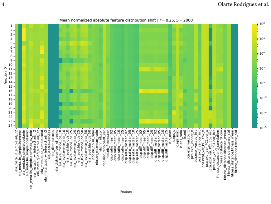
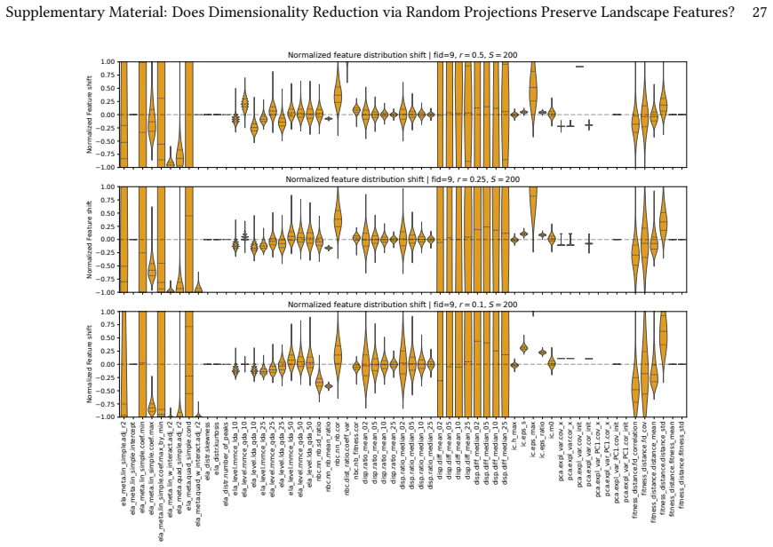
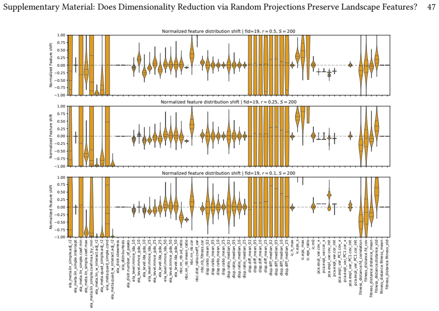
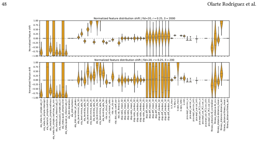
Linear random projections via Gaussian embeddings frequently modify the geometric and topological structures that Exploratory Landscape Analysis depends on, so the resulting feature values cease to be representative of the original high-dimensional problem.
What carries the argument
Direct recomputation of ELA features on the exact same sampled points and objective values, once in the original space and once after Random Gaussian Embedding, followed by numerical comparison across sample budgets and target dimensions.
If this is right
- Most ELA features become unreliable indicators after linear random projection.
- Reduced-space feature values typically do not match the original problem's landscape characteristics.
- Only a small subset of features exhibits comparative stability across projections.
- Even stable features may still encode projection-induced artifacts instead of original landscape traits.
Where Pith is reading between the lines
- High-dimensional algorithm selection that uses ELA should validate feature stability on the concrete problem rather than assume projection preserves information.
- The observed sensitivity points toward testing structure-preserving alternatives such as PCA or manifold learning for future ELA pipelines.
- Practitioners applying ELA to high-dimensional tasks may need to accept higher computational cost or develop projection-aware feature normalizations.
Load-bearing premise
That agreement or disagreement between ELA feature values computed on the same points before and after projection is sufficient to decide whether the reduced features still describe intrinsic properties of the original landscape.
What would settle it
A follow-up experiment on standard benchmark functions that shows the majority of ELA feature classes produce statistically indistinguishable values in the projected space for every tested dimension and sample size.
Figures


read the original abstract
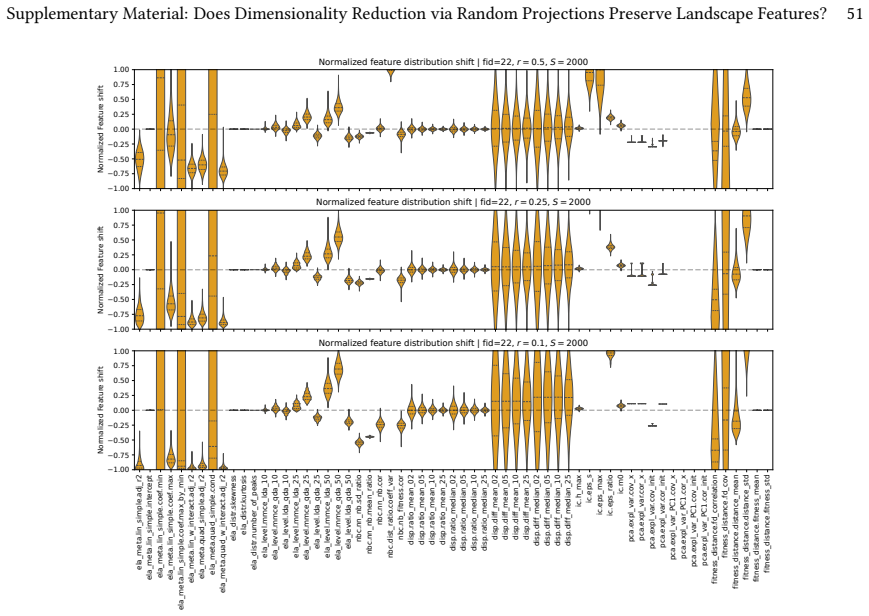
Exploratory Landscape Analysis (ELA) provides numerical features for characterizing black-box optimization problems. In high-dimensional settings, however, ELA suffers from sparsity effects, high estimator variance, and the prohibitive cost of computing several feature classes. Dimensionality reduction has therefore been proposed as a way to make ELA applicable in such settings, but it remains unclear whether features computed in reduced spaces still reflect intrinsic properties of the original landscape. In this work, we investigate the robustness of ELA features under dimensionality reduction via Random Gaussian Embeddings (RGEs). Starting from the same sampled points and objective values, we compute ELA features in projected spaces and compare them to those obtained in the original search space across multiple sample budgets and embedding dimensions. Our results show that linear random projections often alter the geometric and topological structure relevant to ELA, yielding feature values that are no longer representative of the original problem. While a small subset of features remains comparatively stable, most are highly sensitive to the embedding. Moreover, robustness under projection does not necessarily imply informativeness, as apparently robust features may still reflect projection-induced artifacts rather than intrinsic landscape characteristics.
Editorial analysis
A structured set of objections, weighed in public.
Referee Report
Summary. The manuscript investigates whether Exploratory Landscape Analysis (ELA) features remain representative of intrinsic landscape properties when computed on points projected from high-dimensional spaces to lower dimensions via Random Gaussian Embeddings. Starting from identical sampled points and objective values, the authors compare ELA feature values across original and projected spaces for varying sample budgets and embedding dimensions, concluding that most features are sensitive to projection (altering relevant geometric and topological structure) while a small subset appears stable but may reflect projection-induced artifacts rather than intrinsic characteristics.
Significance. If the central empirical findings hold after addressing methodological confounds, the work would be significant for black-box optimization and landscape analysis, as it provides evidence against naive use of dimensionality reduction to enable ELA in high dimensions and highlights the need for careful validation of reduced-space features.
major comments (1)
- [Methodology and Results] The experimental comparison (described in the methodology and results sections) fixes the point set and objective values before applying linear projection and recomputing ELA features. This necessarily increases relative point density in the lower-dimensional space by a factor scaling with the volume ratio, which directly affects density- and neighborhood-dependent ELA feature classes (dispersion, information content, convexity, etc.). No controls are reported to isolate projection-induced density bias from genuine structural alteration, such as density-matched resampling in the target space or validation against analytically known low-dimensional landscapes. This confound is load-bearing for the claim that observed feature shifts indicate loss of intrinsic structure rather than estimator bias.
minor comments (2)
- [Abstract] The abstract and introduction would benefit from explicit enumeration of the test functions, exact original and target dimensions, sample sizes per budget, number of random projections per instance, and any statistical significance testing used to support comparative claims.
- [Results] Figure captions and tables reporting feature stability should include error bars or variability measures across random embeddings to allow readers to assess the reliability of 'stable' versus 'sensitive' classifications.
Simulated Author's Rebuttal
We thank the referee for their detailed and insightful comments on our manuscript. We address the major comment point by point below.
read point-by-point responses
-
Referee: [Methodology and Results] The experimental comparison (described in the methodology and results sections) fixes the point set and objective values before applying linear projection and recomputing ELA features. This necessarily increases relative point density in the lower-dimensional space by a factor scaling with the volume ratio, which directly affects density- and neighborhood-dependent ELA feature classes (dispersion, information content, convexity, etc.). No controls are reported to isolate projection-induced density bias from genuine structural alteration, such as density-matched resampling in the target space or validation against analytically known low-dimensional landscapes. This confound is load-bearing for the claim that observed feature shifts indicate loss of intrinsic structure rather than estimator bias.
Authors: We thank the referee for identifying this important methodological issue. Our experimental setup uses the same set of sampled points and their corresponding objective values in both the original and projected spaces to directly assess the impact of the random projection on the computed ELA features. This design choice simulates the practical application where evaluations obtained in the high-dimensional space are projected for landscape analysis in reduced dimensions. We agree, however, that the increased relative density of points in the lower-dimensional space could influence features that rely on dispersion, neighborhood information, or local convexity, and that this may confound the interpretation of feature changes as purely due to loss of intrinsic structure. To address this concern, we will add control experiments in the revised manuscript, including density-matched resampling in the target space and comparisons with analytically known low-dimensional landscapes. These revisions will help isolate the effects of projection from density bias and strengthen the validity of our conclusions. revision: yes
Circularity Check
No significant circularity; purely empirical feature comparison
full rationale
The manuscript conducts a direct numerical comparison of ELA features computed on identical sampled points and objective values before versus after random Gaussian projection. No derivations, first-principles results, fitted parameters, or predictions are claimed. The central claim rests on observed differences in feature values across dimensions and sample budgets, which does not reduce to any self-referential definition or input by construction. External citations (if present) concern standard ELA definitions and are not load-bearing for any uniqueness or ansatz. Methodological questions about projection-induced density changes are separate from circularity and do not involve any quoted reduction of the reported result to its own inputs.
Axiom & Free-Parameter Ledger
Reference graph
Works this paper leans on
-
[1]
Kirill Antonov, Elena Raponi, Hao Wang, and Carola Doerr. 2022. High Dimen- sional Bayesian Optimization with Kernel Principal Component Analysis. In Parallel Problem Solving from Nature – PPSN XVII (Lecture Notes in Computer Science). 118–131. Does Dimensionality Reduction via Random Projections Preserve Landscape Features? GECCO ’26, July 13–17, 2026, S...
work page 2022
-
[2]
Sanjoy Dasgupta. 1999. Learning mixtures of Gaussians. In40th Annual Sympo- sium on Foundations of Computer Science (Cat. No. 99CB37039). 634–644
work page 1999
- [3]
-
[4]
Nikolaus Hansen, Anne Auger, Raymond Ros, Olaf Mersmann, Tea Tušar, and Dimo Brockhoff. 2021. COCO: A Platform for Comparing Continuous Optimizers in a Black-Box Setting.Optimization Methods and Software36, 1 (2021), 114–144
work page 2021
-
[5]
2009.Real- Parameter Black-Box Optimization Benchmarking 2009: Noiseless Functions Defini- tions
Nikolaus Hansen, Steffen Finck, Raymond Ros, and Anne Auger. 2009.Real- Parameter Black-Box Optimization Benchmarking 2009: Noiseless Functions Defini- tions. Technical Report RR-6829. INRIA
work page 2009
-
[6]
Anja Jankovic and Carola Doerr. 2020. Landscape-aware fixed-budget perfor- mance regression and algorithm selection for modular CMA-ES variants. In Proceedings of the Genetic and Evolutionary Computation Conference (GECCO’20). 841–849
work page 2020
-
[7]
Johnson and Joram Lindenstrauss
William B. Johnson and Joram Lindenstrauss. 1984. Extensions of Lipschitz mappings into a Hilbert space. InContemporary Mathematics. Vol. 26. American Mathematical Society, 189–206
work page 1984
-
[8]
Terry Jones and Stephanie Forrest. 1995. Fitness Distance Correlation as a Measure of Problem Difficulty for Genetic Algorithms. InProceedings of the 6th International Conference on Genetic Algorithms. 184–192
work page 1995
-
[9]
Hoos, Frank Neumann, and Heike Trautmann
Pascal Kerschke, Holger H. Hoos, Frank Neumann, and Heike Trautmann. 2019. Automated Algorithm Selection: Survey and Perspectives.Evolutionary Compu- tation27, 1 (2019), 3–45
work page 2019
-
[10]
Pascal Kerschke, Mike Preuss, Carlos Hernández, Oliver Schütze, Jian-Qiao Sun, Christian Grimme, Günter Rudolph, Bernd Bischl, and Heike Trautmann. 2014. Cell Mapping Techniques for Exploratory Landscape Analysis. InEVOLVE - A Bridge between Probability, Set Oriented Numerics, and Evolutionary Computation V. Vol. 288. Springer International Publishing, 115–131
work page 2014
-
[11]
Pascal Kerschke, Mike Preuss, Simon Wessing, and Heike Trautmann. 2015. Detecting Funnel Structures by Means of Exploratory Landscape Analysis. In Proceedings of the Genetic and Evolutionary Computation Conference (GECCO’15). 265–272
work page 2015
-
[12]
Pascal Kerschke and Heike Trautmann. 2019. Automated Algorithm Selection on Continuous Black-Box Problems By Combining Exploratory Landscape Analysis and Machine Learning.Evolutionary Computation27, 1 (2019), 99–127
work page 2019
-
[13]
Pascal Kerschke and Heike Trautmann. 2019. Comprehensive Feature-Based Landscape Analysis of Continuous and Constrained Optimization Problems Using the R-Package Flacco. InApplications in Statistical Computing: From Music Data Analysis to Industrial Quality Improvement. Springer International Publishing, 93–123
work page 2019
-
[14]
Ana Kostovska, Anja Jankovic, Diederick Vermetten, Jacob de Nobel, Hao Wang, Tome Eftimov, and Carola Doerr. 2022. Per-run algorithm selection with warm- starting using trajectory-based features. InProceedings of the International Con- ference on Parallel Problem Solving from Nature (PPSN’22). 46–60
work page 2022
-
[15]
Monte Lunacek and Darrell Whitley. 2006. The dispersion metric and the CMA evolution strategy. InProceedings of the Genetic and Evolutionary Computation Conference (GECCO’06). 477–484
work page 2006
-
[16]
Leland McInnes and John Healy. 2018. UMAP: Uniform Manifold Approxi- mation and Projection for Dimension Reduction.CoRRabs/1802.03426 (2018). arXiv:1802.03426
work page internal anchor Pith review arXiv 2018
-
[17]
Olaf Mersmann, Bernd Bischl, Heike Trautmann, Mike Preuss, Claus Weihs, and Günter Rudolph. 2011. Exploratory landscape analysis. InProceedings of the Genetic and Evolutionary Computation Conference (GECCO’11). 829–836
work page 2011
-
[18]
Mario Andrés Muñoz, Michael Kirley, and Saman Halgamuge. 2015. Exploratory Landscape Analysis of Continuous Space Optimization Problems Using Infor- mation Content.IEEE Transactions on Evolutionary Computation19, 1 (2015), 74–87
work page 2015
-
[19]
Mario Andrés Muñoz, Michael Kirley, and Kate Smith-Miles. 2022. Analyzing randomness effects on the reliability of exploratory landscape analysis.Natural Computing21, 2 (2022), 131–154
work page 2022
-
[20]
Fabian Pedregosa, Gaël Varoquaux, Alexandre Gramfort, Vincent Michel, Bertrand Thirion, Olivier Grisel, Mathieu Blondel, Peter Prettenhofer, Ron Weiss, Vincent Dubourg, Jake Vanderplas, Alexandre Passos, David Cournapeau, Matthieu Brucher, Matthieu Perrot, and Édouard Duchesnay. 2011. Scikit-learn: Machine Learning in Python.Journal of Machine Learning Re...
work page 2011
-
[21]
Mike Preuss. 2012. Improved Topological Niching for Real-Valued Global Opti- mization. InApplications of Evolutionary Computation. Vol. 7248. Springer-Verlag, 386–395
work page 2012
-
[22]
Elena Raponi, Hao Wang, Mariusz Bujny, Simonetta Boria, and Carola Doerr
-
[23]
InProceedings of the International Conference on Parallel Problem Solving from Nature (PPSN’20)
High Dimensional Bayesian Optimization Assisted by Principal Component Analysis. InProceedings of the International Conference on Parallel Problem Solving from Nature (PPSN’20). 169–183
-
[24]
Quentin Renau, Carola Doerr, Johann Dreo, and Benjamin Doerr. 2020. Ex- ploratory Landscape Analysis is Strongly Sensitive to the Sampling Strategy. InProceedings of the International Conference on Parallel Problem Solving from Nature (PPSN’20). 139–153
work page 2020
-
[25]
Quentin Renau, Johann Dreo, Carola Doerr, and Benjamin Doerr. 2019. Expres- siveness and robustness of landscape features. InProceedings of the Genetic and Evolutionary Computation Conference (GECCO’19) Companion. 2048–2051
work page 2019
-
[26]
Quentin Renau, Johann Dreo, Carola Doerr, and Benjamin Doerr. 2021. To- wards Explainable Exploratory Landscape Analysis: Extreme Feature Selection for Classifying BBOB Functions. InProceedings of the International Conference on Applications of Evolutionary Computation (EvoApplications’21), Held as Part of EvoStar 2021. 17–33
work page 2021
-
[27]
Sobia Saleem, Marcus Gallagher, and Ian Wood. 2019. Direct Feature Evalua- tion in Black-Box Optimization Using Problem Transformations.Evolutionary Computation27, 1 (2019), 75–98
work page 2019
-
[28]
Ryoji Tanabe. 2021. Towards exploratory landscape analysis for large-scale optimization: a dimensionality reduction framework. InProceedings of the Genetic and Evolutionary Computation Conference (GECCO’21). 546–555
work page 2021
-
[29]
Ziyu Wang, Frank Hutter, Masrour Zoghi, David Matheson, and Nando De Freitas
-
[30]
Bayesian Optimization in a Billion Dimensions via Random Embeddings. Journal of Artificial Intelligence Research55 (2016), 361–387. Supplementary Material: Does Dimensionality Reduction via Random Projections Preserve Landscape Features? IVÁN OLARTE RODRÍGUEZ,Leiden Institute of Advanced Computer Science, Leiden University, The Netherlands ANJA JANKOVIC,R...
discussion (0)
Sign in with ORCID, Apple, or X to comment. Anyone can read and Pith papers without signing in.