Quantum Metropolis-Hastings via Penalised Qubitized Walks: Spectral Filtering and Circuit Implementation
Pith reviewed 2026-05-10 10:41 UTC · model grok-4.3
The pith
Quantum Metropolis-Hastings via penalized qubitized walks recovers the correct stationary distribution only after spectral filtering in the circuit model.
A machine-rendered reading of the paper's core claim, the machinery that carries it, and where it could break.
Core claim
The paper establishes that constructing a circuit-level quantum Metropolis-Hastings algorithm from penalized qubitized walks necessitates the inclusion of spectral filtering and other adjustments to the walk dynamics. When these changes are incorporated, the simulated quantum circuit produces the same stationary distribution as the classical algorithm; without them, the distribution is incorrect.
What carries the argument
The spectral-filtered penalized qubitized walk, which serves as the quantum operator that encodes the Metropolis-Hastings transition probabilities while operating within the constraints of a quantum circuit.
If this is right
- The stationary distribution of the quantum algorithm matches the classical one when filtering is applied.
- Quantum walks can be used for accelerated Monte Carlo sampling in circuit-based quantum computers.
- The approach highlights specific engineering steps needed for practical quantum Markov chain methods.
- Limitations remain in scaling to large systems due to circuit complexity.
Where Pith is reading between the lines
- Techniques like spectral filtering could be generalized to enhance other quantum walk algorithms for sampling.
- Implementation on current quantum simulators would allow verification of the distribution matching beyond ideal cases.
- This could open paths to quantum-enhanced Bayesian inference in machine learning models.
Load-bearing premise
The modifications to the qubitized walk, including penalization and spectral filtering, can be realized in a quantum circuit without altering the target stationary distribution of the Metropolis-Hastings algorithm.
What would settle it
Performing a circuit simulation of the quantum walk without applying spectral filtering and checking whether the output state probabilities differ from the analytically computed Metropolis-Hastings stationary distribution.
Figures
read the original abstract
The Metropolis-Hastings algorithm is a cornerstone of Markov Chain Monte Carlo methods, underpinning a wide range of applications in computational physics, Bayesian inference, and machine learning. Quantum variants of Metropolis-Hastings promise accelerated mixing through quantum walks, but their practical realisation remains challenging. In this work, we construct and simulate an explicit circuit level implementation of a quantum Metropolis-Hastings algorithm based on the framework introduced by Claudon \emph{et al.} (arXiv:2506.11576). We present the full quantum workflow required to prepare a stationary distribution, including a number of modifications required to make the algorithm implementable in a realistic quantum circuit model. Our results demonstrate that these modifications are essential to recover the correct stationary behaviour and highlight both the potential and current limitations of quantum Metropolis-Hastings algorithms, which are expected to become practically relevant in the fault tolerant quantum computing regime.
Editorial analysis
A structured set of objections, weighed in public.
Referee Report
Summary. The manuscript constructs an explicit circuit-level implementation of a quantum Metropolis-Hastings algorithm by adapting the penalized qubitized walk framework of Claudon et al., incorporating spectral filtering and other modifications to enable realization in a realistic quantum circuit model. Numerical simulations on small instances are presented to demonstrate that these modifications are essential for recovering the target stationary (Boltzmann) distribution.
Significance. If the modifications preserve the intended stationary distribution, the work supplies a concrete workflow and identifies practical obstacles for quantum MCMC algorithms, which could become relevant in the fault-tolerant regime. The emphasis on circuit adaptations and their necessity offers guidance for future implementations, though the absence of analytical guarantees restricts the result's immediate generality.
major comments (1)
- No derivation is given showing that the effective walk operator (after penalization, spectral filtering, and circuit approximations) continues to satisfy detailed balance or has the target Boltzmann distribution as its unique stationary state. The central claim that the modifications recover the correct stationary behaviour therefore rests entirely on numerical simulations of small systems; any perturbation to the null space would shift the distribution without necessarily being visible in those instances.
minor comments (2)
- Simulation results lack error bars, full circuit diagrams, and quantitative metrics (e.g., fidelity or distance to target distribution), limiting independent verification of the claim that the modifications are essential.
- Notation and operator definitions carried over from the cited prior work would benefit from explicit re-statement to improve standalone readability.
Simulated Author's Rebuttal
We thank the referee for the careful reading and for recognizing the practical value of the circuit workflow and identified obstacles. We address the major comment point by point below.
read point-by-point responses
-
Referee: No derivation is given showing that the effective walk operator (after penalization, spectral filtering, and circuit approximations) continues to satisfy detailed balance or has the target Boltzmann distribution as its unique stationary state. The central claim that the modifications recover the correct stationary behaviour therefore rests entirely on numerical simulations of small systems; any perturbation to the null space would shift the distribution without necessarily being visible in those instances.
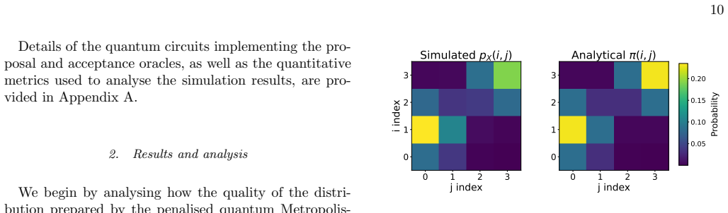
Authors: We agree that the manuscript provides no complete analytical derivation proving that the effective walk operator after penalization, spectral filtering, and circuit approximations exactly satisfies detailed balance or possesses the target Boltzmann distribution as its unique stationary state. The central claim is indeed supported by numerical simulations on small systems, where the effective operator can be exactly diagonalized to verify recovery of the stationary distribution (to high accuracy) only when the modifications are included. We will revise the manuscript by adding a dedicated subsection that supplies a construction-based argument: the penalization is engineered to suppress components outside the target subspace while spectral filtering projects onto the low-energy eigenspace, and the circuit approximations are controlled (small-angle or perturbative). A brief perturbation analysis will be included to bound the shift in the stationary state for the error levels considered, addressing visibility concerns by showing that deviations scale with the approximation error and remain detectable even in the simulated regimes. This strengthens the presentation without claiming a full rigorous proof, which lies outside the current scope focused on explicit circuit realization. revision: partial
Circularity Check
No circularity detected; construction relies on external framework plus independent numerical validation
full rationale
The paper adapts the penalized qubitized walk framework from the externally cited Claudon et al. (arXiv:2506.11576) and introduces circuit-level modifications whose effect on the stationary distribution is checked via explicit small-system simulations. No step reduces a claimed result to a fitted parameter, self-citation, or definitional renaming; the central demonstration that the modifications recover the target Boltzmann distribution is presented as an empirical outcome rather than an algebraic identity with the inputs. The derivation chain therefore remains self-contained against external benchmarks.
Axiom & Free-Parameter Ledger
axioms (1)
- domain assumption Standard quantum circuit model and fault-tolerant quantum computing assumptions hold for the target implementation.
Reference graph
Works this paper leans on
-
[1]
How- ever, when a finite number of ancilla qubits is used, the resulting filter is not exact. Instead, it realises a Dirichlet kernel [22], corresponding to a sharply peaked response at phase 0 with small side lobes. These side lobes allow eigenstates with nearby phases to pass the filter with a probability that depends on the number of ancillas used: P r...
-
[2]
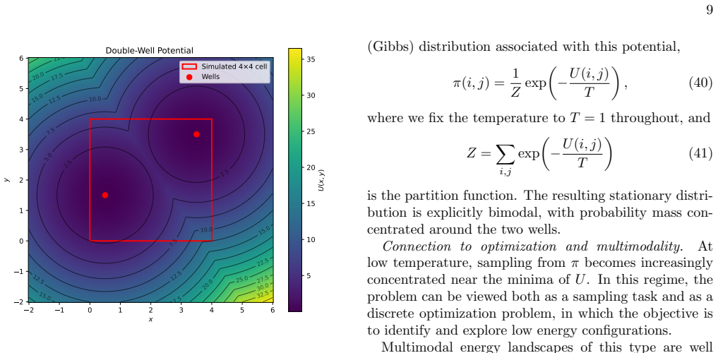
Model and target distribution To illustrate the behaviour of the quantum Metropolis- Hastings algorithm in the presence of multimodality, we consider a simple but representative double well energy landscape defined on a finite two-dimensional lattice (see Fig. 3). The figure provides a continuous visualization of the underlying landscape for geometric int...
-
[3]
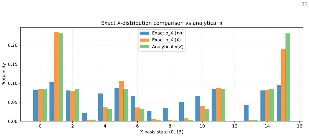
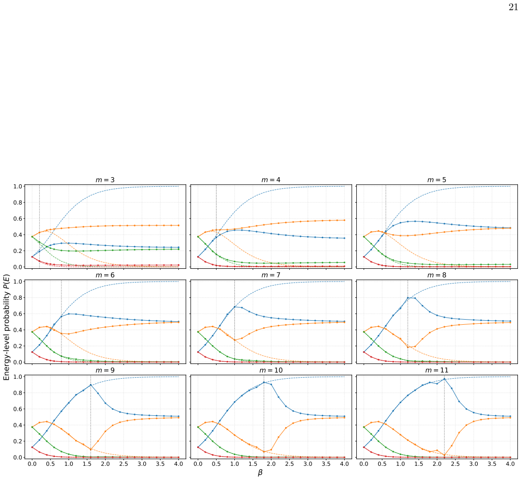
Results and analysis We begin by analysing how the quality of the distri- bution prepared by the penalised quantum Metropolis- Hastings algorithm depends on the numbermof precision qubits used in the QPE filter. The parametermcontrols the spectral resolution of the filtering step and thus di- rectly affects how accurately the stationary distribution can b...
-
[4]
Model and target distribution The Ising model is a paradigmatic system in statisti- cal physics and serves as a standard benchmark for sam- pling algorithms. Its simplicity, combined with temper- ature dependent correlations, makes it a natural testbed for analysing both classical and quantum Markov chain Monte Carlo methods. State space and proposal geom...
-
[5]
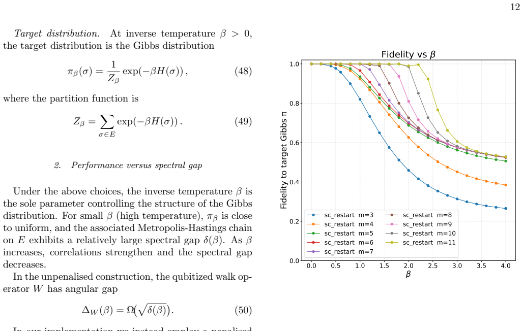
Performance versus spectral gap Under the above choices, the inverse temperatureβis the sole parameter controlling the structure of the Gibbs distribution. For smallβ(high temperature),π β is close to uniform, and the associated Metropolis-Hastings chain onEexhibits a relatively large spectral gapδ(β). Asβ increases, correlations strengthen and the spectr...
-
[6]
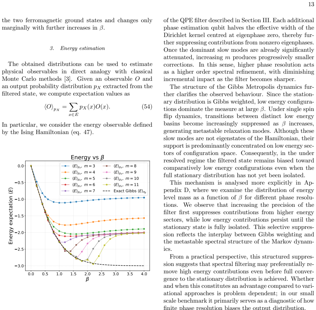
Energy estimation The obtained distributions can be used to estimate physical observables in direct analogy with classical Monte Carlo methods [3]. Given an observableOand an output probability distributionp X extracted from the filtered state, we compute expectation values as ⟨O⟩pX = X x∈E pX(x)O(x).(54) In particular, we consider the energy observable d...
-
[7]
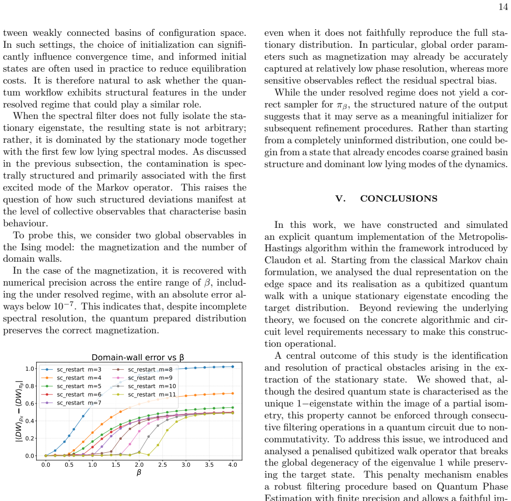
Basin structure In realistic implementations, resource limitations may prevent the algorithm from operating in the fully re- solved regime where we have enough precision ancillas to filter the target distribution. Although in the present work this limitation arises from classical simulation con- straints, similar restrictions are expected in larger scale ...
-
[8]
E.W. Larsen. An overview of neutron transport problems and simulation techniques. InComputational Methods in Transport, pages 513–534, 2006
work page 2006
-
[9]
Kalos and P.A Whitlock.Monte Carlo Methods
M.H. Kalos and P.A Whitlock.Monte Carlo Methods. WILEY-VCH Verlag GmbH & Co. KGaA, second edi- tion, 2008
work page 2008
-
[10]
K. Choo, A. Mezzacapo, and G. Carleo. Fermionic neural-network states for ab-initio electronic structure. Nature Communications, 11(1), 2020
work page 2020
-
[11]
J. W. T. Keeble, M. Drissi, A. Rojo-Franc` as, B. Juli´ a- D´ ıaz, and A. Rios. Machine learning one-dimensional spinless trapped fermionic systems with neural-network quantum states.Physical Review A, 108(6), 2023
work page 2023
-
[12]
J.P. Kaipio and E. Somersalo.Statistical and Computa- tional Inverse Problems. Springer, first edition, 2004
work page 2004
- [13]
-
[14]
G. Roberts and J. Rosenthal. General state space markov chains and mcmc algorithms.Probability Surveys, 1, April 2004
work page 2004
-
[15]
K. Wu, S. Schmidler, and Y. Chen. Minimax mixing time of the metropolis-adjusted langevin algorithm for log-concave sampling.Journal of Machine Learning Re- search, 23, 2022
work page 2022
- [16]
-
[17]
Q. Zhou and H. Chang. Complexity analysis of bayesian learning of high-dimensional dag models and their equiv- alence classes.The Annals of Statistics, 51, 2021
work page 2021
-
[18]
M. Szegedy. Quantum speed-up of markov chain based algorithms. In45th Annual IEEE Symposium on Foun- dations of Computer Science, pages 32–41, 2004
work page 2004
-
[19]
D. Levin and Y. Peres.Markov Chains and Mixing Times. American Mathematical Society, second edition, 2009
work page 2009
-
[20]
J. Lemieux, B. Heim, D. Poulin, K. Svore, and M. Troyer. Efficient quantum walk circuits for metropolis-hastings algorithm.Quantum, 4, June 2020
work page 2020
-
[21]
K. Temme, T.J. Osborne, K.G.H. Vollbrecht, D. Poulin, and F. Verstraete. Quantum metropolis sampling.Na- ture, 471(7336), 2011
work page 2011
- [22]
-
[23]
B. Claudon, P. Rodenas-Ruiz, J.P. Piquemal, and P. Monmarch´ e. Quantum circuits for the metropolis- hastings algorithm, 2025. 16
work page 2025
-
[24]
D.S. Alonso and O. Al-Ghattas. A first course in monte carlo methods, 2024
work page 2024
-
[25]
C. S¨ underhauf. Generalized quantum singular value transformation, 2023
work page 2023
-
[26]
F. Magniez, A. Nayak, J. Roland, and M. Santha. Search via quantum walk.SIAM Journal on Computing, 40(1), 2011
work page 2011
- [27]
-
[28]
J.M. Martyn, Z.M. Rossi, A.K. Tan, and I.L. Chuang. Grand unification of quantum algorithms.PRX Quan- tum, 2(4), 2021
work page 2021
-
[29]
A.M. Bruckner, J.B. Bruckner, and B.S. Thomson.Real Analysis. Prentice-Hall, first edition, 1997
work page 1997
-
[30]
S. Parker and M.B. Plenio. Efficient factorization with a single pure qubit and logn mixed qubits.Physical Review Letters, 85(14), 2000
work page 2000
-
[31]
M. Carrasco-Arango. Quantum metropolis hastings: Circuit implementation, 2026.https://github.com/ bsc-wdc/q-mcmc. Appendix A: Circuit implementations In this appendix we present the quantum circuits implementing the penalised version of the quantum Metropolis-Hastings algorithm. The full implementation, including circuit generation and simulation code, is...
work page 2026
-
[32]
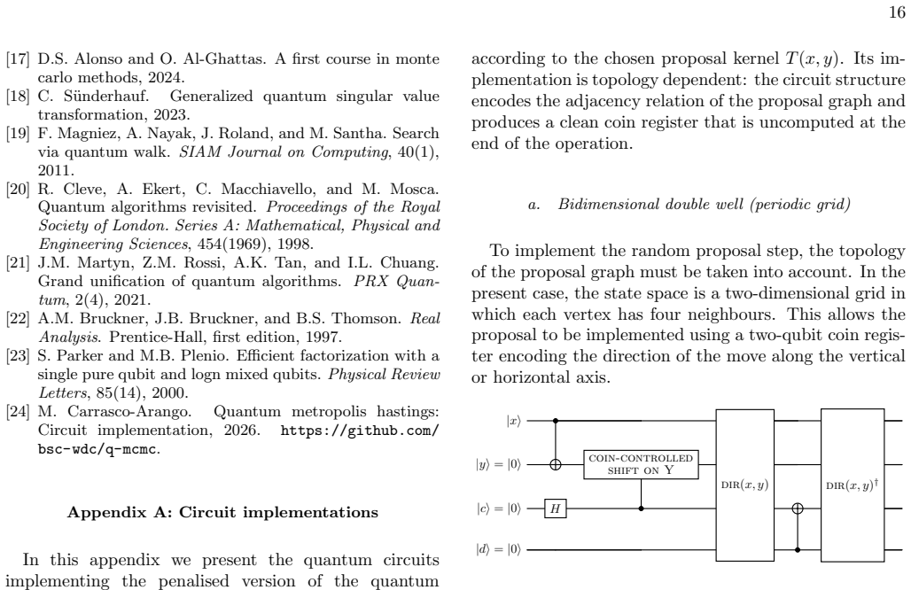
Proposal oracleO T The proposal oracleO T prepares, for each current state x, a coherent superposition over neighbouring statesy according to the chosen proposal kernelT(x, y). Its im- plementation is topology dependent: the circuit structure encodes the adjacency relation of the proposal graph and produces a clean coin register that is uncomputed at the ...
-
[33]
11: Quantum circuit implementing the acceptance op- erator ofP,O A
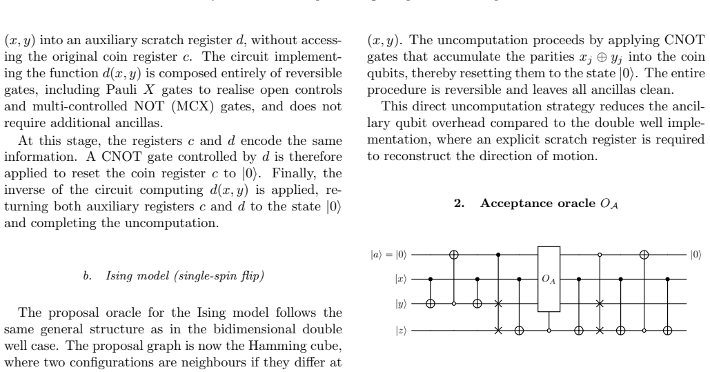
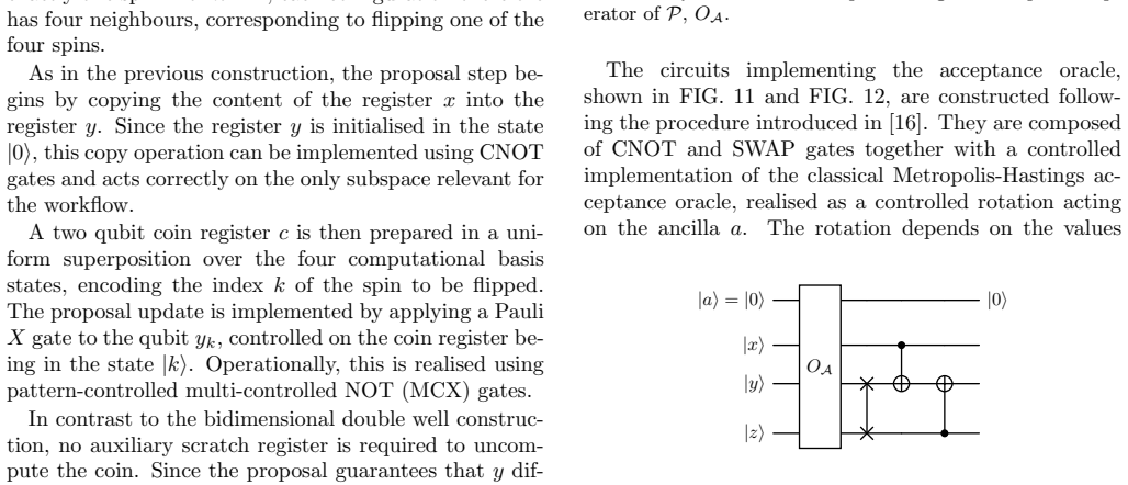
Acceptance oracleO A |a⟩=|0⟩ OA |0⟩ |x⟩ |y⟩ |z⟩ FIG. 11: Quantum circuit implementing the acceptance op- erator ofP,O A. The circuits implementing the acceptance oracle, shown in FIG. 11 and FIG. 12, are constructed follow- ing the procedure introduced in [16]. They are composed of CNOT and SWAP gates together with a controlled implementation of the class...
-
[34]
As discussed in the main text, however,W is not used directly
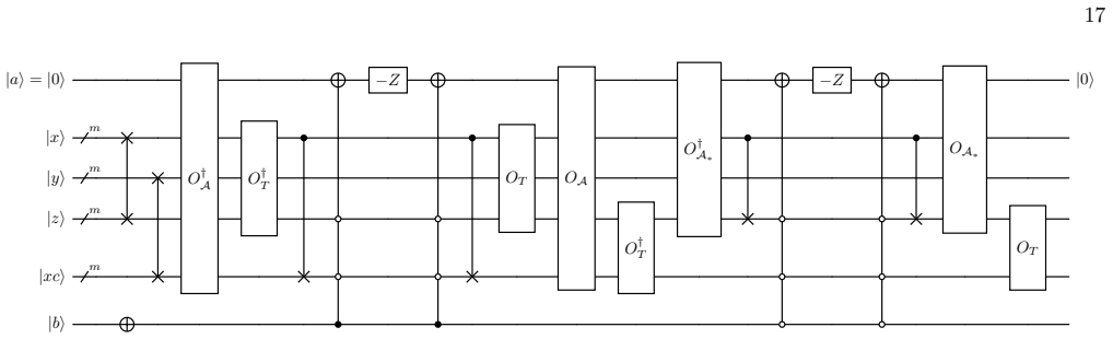
Penalised qubitized walkV Given the proposal and acceptance oracles, we can con- struct the PUEs required to implement the qubitized walkW. As discussed in the main text, however,W is not used directly. Instead, we work with a penalised versionV= Π⊠ +e iφ(Id−Π ⊠) W, as introduced in section III. Since projectors cannot be implemented directly in a quantum...
-
[35]
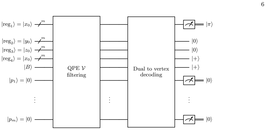
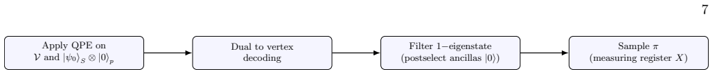
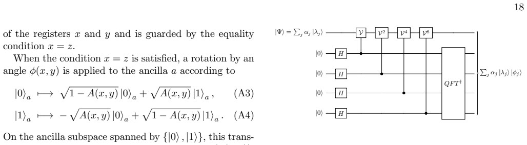
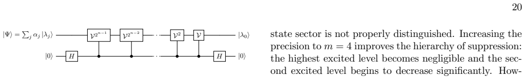
Quantum Phase Estimation The eigenstate filtering step is implemented using the Quantum Phase Estimation algorithm, whose circuit is shown in Fig. 13. The QPE is applied to the penalised |Ψ⟩= ∑ jαj |λj⟩ V V 2 V 4 V 8 ∑ jαj |λj⟩ |ϕj⟩ |0⟩ H QFT † |0⟩ H |0⟩ H |0⟩ H FIG. 13: Quantum circuit implementing the Quantum Phase Estimation (QPE) algorithm. qubitized ...
-
[36]
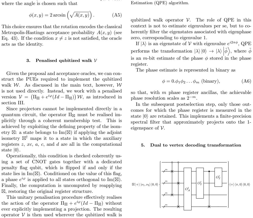
Dual to vertex decoding transformation m m m m ⊠|+⟩ |ν1,ν2⟩ |0,0⟩ |+⟩ |π,0⟩ |0,0⟩ O† A O† T O† T FIG. 14: Quantum circuit implementing the final transforma- tion on the ancillaband the four main registers. After the QPE based filtering step, the resulting quan- tum state is close to the 1−eigenstate of the penalised qubitized walk operatorV. When the pena...
-
[37]
Classical fidelity To quantify the global overlap between the prepared distributionp X and the target distributionπ, we use the classical fidelity F(p X , π) = X x∈E p pX(x)π(x) !2 .(B1) This quantity takes values in [0,1], withF(p X , π) = 1 if and only ifp X =π. The classical fidelity is symmet- ric, insensitive to small local fluctuations, and provides...
-
[38]
Total variation distance As a complementary metric, we consider the total vari- ation distance dTV(pX , π) = 1 2 X x∈E |pX(x)−π(x)|.(B2) The total variation distance has a clear operational inter- pretation as the maximum probability of distinguishing the two distributions with a single sample. Unlike the fidelity, it is sensitive to local discrepancies a...
-
[39]
Local basin mass In order to analyse the structure of deviations between pX andπin Section III, we additionally consider the probability mass assigned to local neighbourhoods of the energy minima. Given a minimumx ⋆ = (i ⋆, j⋆)∈E and a radiusr≥0, we define a local basin as theL ∞ neighbourhood B∞(x⋆, r) ={(i, j)∈E| |i−i ⋆| ≤r,|j−j ⋆| ≤r}. (B3) For a set o...
discussion (0)
Sign in with ORCID, Apple, or X to comment. Anyone can read and Pith papers without signing in.