arxiv: 2604.16932 · v1 · submitted 2026-04-18 · 📊 stat.ML · cs.LG

Recognition: unknown

Neighbor Embedding for High-Dimensional Sparse Poisson Data

Noga Mudrik , Adam S. Charles

Authors on Pith no claims yet

Pith reviewed 2026-05-10 06:46 UTC · model grok-4.3

classification 📊 stat.ML cs.LG

keywords Poisson datastochastic neighbor embeddingdimensionality reductionKL divergenceHellinger distancesparse count dataneural spike data

0 comments

The pith

p-SNE embeds high-dimensional sparse count data by using KL divergence between Poisson distributions to measure dissimilarity.

A machine-rendered reading of the paper's core claim, the machinery that carries it, and where it could break.

The paper develops p-SNE, a nonlinear embedding method built specifically for high-dimensional data that follow Poisson distributions, such as word counts in documents or spike counts in neural recordings. Existing techniques like t-SNE rely on Euclidean geometry that does not match the discrete and sparse character of low-rate count observations, leading to distorted representations of structure. p-SNE instead computes neighbor probabilities from the Kullback-Leibler divergence between Poisson distributions and optimizes the low-dimensional layout with Hellinger distance. When this approach works, it recovers interpretable patterns such as weekday cycles in email traffic, topical clusters among research papers, and stimulus-related gradients in brain activity.

Core claim

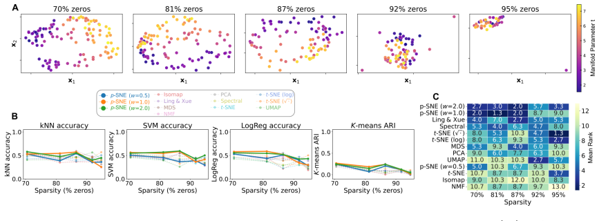
p-SNE is a nonlinear neighbor embedding method designed around the Poisson structure of count data, using KL divergence between Poisson distributions to measure pairwise dissimilarity and Hellinger distance to optimize the embedding. Tests on synthetic Poisson data and real datasets demonstrate recovery of weekday patterns in email communication, research area clusters in OpenReview papers, and temporal drift together with stimulus gradients in neural spike recordings.

What carries the argument

p-SNE, a stochastic neighbor embedding variant that substitutes Poisson KL divergence for Euclidean distances when defining neighbor probabilities and employs Hellinger distance during layout optimization.

If this is right

Synthetic Poisson data with known cluster structure is recovered in the low-dimensional embedding.
Email count matrices separate into weekday patterns without additional supervision.
Research paper abstracts form clusters aligned with topical areas.
Neural spike counts reveal both slow temporal drift and stimulus-driven gradients in the same embedding.

Where Pith is reading between the lines

These are editorial extensions of the paper, not claims the author makes directly.

The same Poisson-based dissimilarity could be substituted into other embedding or clustering algorithms that currently use Euclidean distances.
When count data exhibit overdispersion, replacing the Poisson KL term with a negative-binomial version might preserve the same advantages.
Downstream supervised models trained on the p-SNE coordinates may achieve higher accuracy on count-based prediction tasks than models trained on Euclidean embeddings.

Load-bearing premise

The assumption that KL divergence between Poisson distributions is the right measure of pairwise dissimilarity for preserving meaningful structure in sparse count data.

What would settle it

Applying p-SNE to synthetic data generated from two well-separated Poisson rate vectors and finding that the resulting embedding mixes the two groups instead of keeping them distinct.

Figures

Figures reproduced from arXiv: 2604.16932 by Adam S. Charles, Noga Mudrik.

**Figure 1.** Figure 1: Overview of p-SNE. (A) Euclidean distance assigns the same value (1.73) to both pairs (xn1 vs. xn2 and xn1 vs. xn3 ), while Poisson KL divergence distinguishes them (0.05 vs. 0.92), since differences at low counts (pink arrows) alter the implied Poisson distribution more than equal-sized differences at high counts (blue arrows).(B) p-SNE computes pairwise Poisson KL dissimilarities from a count matrix Y ∈ … view at source ↗

**Figure 2.** Figure 2: Angular Embedding: p-SNE recovers group structure on a Poisson count benchmark. (A) Raw count matrix Y ∈ Z 60×40 ≥0 , sorted by group label. (B) Count distribution per group; vertical lines indicate per-group means. (C) Mean rank across classification metrics (kNN, SVM, k-means ARI) for p-SNE and nine baselines; lower rank is better. (D) 3D embeddings colored by group label. p-SNE (w=1.0) achieves the best… view at source ↗

**Figure 3.** Figure 3: Effect of sparsity on embedding quality (Angular Embedding, M = 40 features). (A) p-SNE (w=1.0) 2D embeddings at five sparsity levels, generated by rescaling the Poisson rate parameters. Group separation degrades gradually but remains visible up to 74% zeros. (B) Classification and clustering metrics as a function of sparsity for p-SNE (w ∈ {0.5, 1.0, 2.0}) and ten baselines, evaluated on the 2D embedding… view at source ↗

**Figure 4.** Figure 4: Sparse Sequential Embedding: p-SNE recovers manifold structure under high sparsity. (A) Raw count matrix Y ∈ Z 119×30 ≥0 , sorted by ground-truth manifold parameter t. (B) Count distribution per group; vertical lines indicate per-group means. (C) Spearman correlation between embedding dimensions and t for p-SNE and nine baselines; higher is better. p-SNE (w=2.0) ranks second overall, outperforming all t-SN… view at source ↗

**Figure 5.** Figure 5: Sparsity sweep on the Sparse Sequential Embedding dataset. (A) p-SNE embeddings (w=2.0) colored by the continuous manifold parameter t, at five sparsity levels (70%-95% zeros). The smooth color gradient indicates that p-SNE recovers the latent manifold structure even at extreme sparsity. (B) Classification and clustering metrics as a function of sparsity for p-SNE variants (solid) and baselines (dashed). … view at source ↗

**Figure 6.** Figure 6: Email sender count data. (A) Raw count matrix Y ∈ Z 153×150 ≥0 (days×senders), sorted by label: Tuesday, Saturday, and Sunday. (B) Count value distribution, stratified by weekday (red) and weekend (blue). (C) SVM (RBF kernel) classification accuracy on 3D embeddings (5-fold crossvalidation, for visualization here Tuesday vs. weekend; full data in Fig. S14). p-SNE achieves the highest accuracy (0.843). (D)… view at source ↗

**Figure 7.** Figure 7: Word-count experiment (OpenReview). 350 academic papers from ICLR 2024/2025 and TMLR, represented as word-count vectors (350 paper samples (5 research areas with 70 papers each) × 100 word features). (A) Raw count matrix Y sorted by research area, showing sparse Poisson structure with area-specific word usage patterns. (B) Count value distribution (81.7% zeros, mean count 0.29). (C) 3D embeddings colored b… view at source ↗

**Figure 8.** Figure 8: Neuroscience experiment: neural spike count data from the Allen Brain Observatory. (A) Spike count distribution stratified by stimulus orientation (8 classes, color-coded). Distributions overlap substantially across orientations, reflecting the difficulty of the classification task. (B) Spike count distribution stratified by temporal frequency (5 classes). Lower frequencies (1-2 Hz) produce slightly highe… view at source ↗

read the original abstract

Across many scientific fields, measurements often represent the number of times an event occurs. For example, a document can be represented by word occurrence counts, neural activity by spike counts per time window, or online communication by daily email counts. These measurements yield high-dimensional count data that often approximate a Poisson distribution, frequently with low rates that produce substantial sparsity and complicate downstream analysis. A useful approach is to embed the data into a low-dimensional space that preserves meaningful structure, commonly termed dimensionality reduction. Yet existing dimensionality reduction methods, including both linear (e.g., PCA) and nonlinear approaches (e.g., t-SNE), often assume continuous Euclidean geometry, thereby misaligning with the discrete, sparse nature of low-rate count data. Here, we propose p-SNE (Poisson Stochastic Neighbor Embedding), a nonlinear neighbor embedding method designed around the Poisson structure of count data, using KL divergence between Poisson distributions to measure pairwise dissimilarity and Hellinger distance to optimize the embedding. We test p-SNE on synthetic Poisson data and demonstrate its ability to recover meaningful structure in real-world count datasets, including weekday patterns in email communication, research area clusters in OpenReview papers, and temporal drift and stimulus gradients in neural spike recordings.

Editorial analysis

A structured set of objections, weighed in public.

Desk editor's note, referee report, simulated authors' rebuttal, and a circularity audit. Tearing a paper down is the easy half of reading it; the pith above is the substance, this is the friction.

Desk Editor's Note private letter to a colleague

p-SNE adapts neighbor embedding to Poisson count data via KL dissimilarities and Hellinger optimization, with claimed recovery of structure in synthetic and real count sets like spikes and emails.

read the letter

The main point on this paper is that it introduces p-SNE, a direct tweak to stochastic neighbor embedding that replaces Euclidean assumptions with Poisson KL divergence for high-dimensional pairwise distances and Hellinger distance for the low-dimensional layout. That targets a real mismatch in sparse count data from events like word occurrences or neural spikes, where standard t-SNE can distort low-rate structure.

Referee Report

0 major / 3 minor

Summary. The manuscript introduces p-SNE, a nonlinear neighbor embedding method for high-dimensional sparse Poisson count data. High-dimensional pairwise dissimilarities are measured via KL divergence between Poisson distributions, while the low-dimensional embedding is optimized using Hellinger distance. The authors evaluate the approach on synthetic Poisson data and demonstrate recovery of structure in three real-world count datasets: weekday patterns from email counts, research-area clusters from OpenReview paper counts, and temporal/stimulus gradients from neural spike recordings.

Significance. If the reported structure recovery holds under quantitative scrutiny, p-SNE would fill a methodological gap by respecting the discrete, low-rate Poisson geometry of count data rather than imposing Euclidean assumptions. This could improve embeddings for text, neuroscience, and network data where standard t-SNE or PCA often distort sparse count structure. The multi-domain empirical examples provide initial evidence of practical relevance.

minor comments (3)

The abstract and introduction claim superior recovery of structure, but no quantitative metrics (e.g., neighborhood preservation, trustworthiness, or reconstruction error) are summarized in the provided text; adding a comparison table against t-SNE, UMAP, and Poisson PCA would strengthen the central claim.
Section describing the optimization (likely §3 or §4) should clarify the precise form of the Hellinger-based cost function and any gradient approximations used, as the switch from KL to Hellinger is load-bearing for the method's distinction from standard SNE.
The real-data experiments would benefit from explicit statements of the Poisson rate assumptions and any preprocessing (e.g., thresholding or normalization) applied to the count matrices, to allow reproducibility.

Simulated Author's Rebuttal

0 responses · 0 unresolved

We thank the referee for their supportive summary of the manuscript and for recommending minor revision. We appreciate the recognition that p-SNE addresses a methodological gap for sparse Poisson count data and that the empirical examples across email, OpenReview, and neural spike datasets provide initial evidence of relevance. We are pleased that the approach is viewed as potentially improving upon standard t-SNE or PCA for discrete, low-rate count data.

Circularity Check

0 steps flagged

No significant circularity detected

full rationale

The paper introduces p-SNE as a novel construction that defines pairwise dissimilarities via KL divergence on Poisson distributions and optimizes embeddings with Hellinger distance. No equations or steps in the abstract or described method reduce by construction to fitted parameters, self-referential predictions, or load-bearing self-citations. Empirical tests on synthetic Poisson data and independent real-world count datasets (email, papers, neural spikes) function as external validation rather than inputs that force the claimed outcomes. The derivation chain remains self-contained against the stated assumptions.

Axiom & Free-Parameter Ledger

0 free parameters · 1 axioms · 0 invented entities

The central claim rests on treating data as Poisson distributed and on the suitability of KL divergence and Hellinger distance for structure preservation; no free parameters or invented entities are described in the abstract.

axioms (1)

domain assumption Measurements represent counts that approximate a Poisson distribution with low rates leading to sparsity.
Explicitly stated in the abstract as the data type the method targets.

pith-pipeline@v0.9.0 · 5508 in / 1240 out tokens · 46917 ms · 2026-05-10T06:46:02.967476+00:00 · methodology

discussion (0)

Reference graph

Works this paper leans on

8 extracted references · 4 canonical work pages · 1 internal anchor

[1]

arXiv preprint arXiv:1910.00204 , year=

Ehsan Amid and Manfred K Warmuth. Trimap: Large-scale dimensionality reduction using triplets. arXiv preprint arXiv:1910.00204,

work page arXiv 1910
[2]

UMAP: Uniform Manifold Approximation and Projection for Dimension Reduction

Leland McInnes, John Healy, and James Melville. Umap: Uniform manifold approximation and projection for dimension reduction.arXiv preprint arXiv:1802.03426,

work page internal anchor Pith review arXiv
[3]

Multi-integration of labels across categories for component identification (milcci).arXiv preprint arXiv:2602.04270,

Noga Mudrik, Yuxi Chen, Gal Mishne, and Adam S Charles. Multi-integration of labels across categories for component identification (milcci).arXiv preprint arXiv:2602.04270,

work page arXiv
[4]

Multi- way multislice phate: Visualizing hidden dynamics of rnns through training.arXiv preprint arXiv:2406.01969,

Jiancheng Xie, Lou C Kohler Voinov, Noga Mudrik, Gal Mishne, and Adam Charles. Multi- way multislice phate: Visualizing hidden dynamics of rnns through training.arXiv preprint arXiv:2406.01969,

work page arXiv
[5]

Each gradient descent iteration involves updating the Student-t kernel matrixQand computing the gradient (Eq

operations (softmax normalization and symmetrization). Each gradient descent iteration involves updating the Student-t kernel matrixQand computing the gradient (Eq. S7), both of which costO(N 2P) wherePis the embedding dimensionality. OverK iterations, the total cost isO(N 2M+KN 2P). SinceM≫Pin all our experiments, the distance matrix computation dominate...

2022
[6]

20 , h ∗ m = 10· ⌊m/20⌋ 2 (S17) Neurons with adjacent indices thus have nearby preferred positions alongt. Firing rates and spike counts.The firing rate of neuronmon trialidepends on the distance between the stimulus position (t i, hi) and the neuron’s preferred position (t ∗ m, h∗ m): λi,m =λ bias +λ peak exp −∆t2 i,m 2 − ∆h2 i,m 20 ! (S18) 29 Figure S14...

2022
[7]

30 Table S3: Wall-clock runtime (seconds) ford= 3 embedding dimensions on both synthetic datasets

+ 1.5), h∼Uniform(0,5) (S19) For each class, we draw 30 stimulus positions (t i, hi), yieldingN= 120 trials (one all-zero sample was removed, giving 119). 30 Table S3: Wall-clock runtime (seconds) ford= 3 embedding dimensions on both synthetic datasets. Method Angular Embedding Sparse Sequential PCA 0.18 0.04 NMF 0.21 0.07 Spectral 0.27 0.09 Isomap 0.59 0...

2022
[8]

person A

25 , h ∗ m = 5.0· ⌊m/25⌋ 2 (S20) Firing rates and spike counts.The firing rate of neuronmon trialiis: λi,m =λ bias +λ peak exp − d2 i,m 3 ! (S21) whered i,m = p (ti −t ∗m)2 + (hi −h ∗m)2 is the Euclidean distance between the stimulus and the neuron’s preferred position. We setλ bias = 0.1 andλ peak = 2.5, so rates range from 0.1 to 2.6. The observed spike...

2022