Recognition: no theorem link
Contagion or Macroeconomic Fluctuations? Identifiability in Aggregated Default Data
Pith reviewed 2026-05-12 01:46 UTC · model grok-4.3
The pith
Most annual default clustering arises from cross-year shifts in conditions rather than within-year contagion after aggregation.
A machine-rendered reading of the paper's core claim, the machinery that carries it, and where it could break.
Core claim
Under the hierarchical specification, cross-year movements in default conditions account for most variation in annual default counts, leaving threshold-type contagion with no separable stable component while cumulative contagion retains a small but detectable persistent element in variance decomposition and tail behavior.
What carries the argument
Variance decomposition and tail comparison across the Lo-Davis cumulative contagion model, Torri threshold contagion model, and Vasicek common-factor model, first under i.i.d. assumptions and then under a hierarchical model that lets default probability vary by year.
If this is right
- Threshold contagion is absorbed into macro variation and cannot be recovered from aggregate counts.
- Cumulative contagion leaves a small stable component that survives aggregation.
- The Vasicek common-factor structure fits observed clustering better than either contagion model under i.i.d. conditions.
- Identifiability of contagion from coarse data depends on the precise form of the interaction mechanism.
Where Pith is reading between the lines
- Finer-grained data on individual defaults or timing within years would be needed to separate contagion from macro effects more reliably.
- Risk models that rely solely on aggregate counts may attribute cumulative-contagion effects to macro shocks instead.
- The same identifiability limits may apply to other aggregated contagion settings such as interbank lending or supply-chain defaults.
Load-bearing premise
The three chosen dependence structures are the only relevant ones, and letting default probability change freely each year fully captures macroeconomic heterogeneity without leftover confounding.
What would settle it
After fitting the hierarchical macro component to real annual default counts, check whether the remaining variance and extreme tail quantiles match the small persistent residual predicted by the Lo-Davis model or the zero residual predicted by the Torri model.
Figures


read the original abstract
Can contagion be inferred from aggregated default data? We study this as a problem of identifiability, asking whether contagion generates components in default count distributions that remain distinct from those induced by macroeconomic fluctuations. We compare three dependence structures: cumulative contagion in the Lo-Davis model, threshold-type contagion in the Torri model, and common-factor dependence in the Vasicek model. Under an i.i.d. specification, the Vasicek model provides the best overall fit, especially in the tail, indicating that a smooth mixture structure captures annual default clustering more effectively than threshold-type contagion at the aggregate level. We then allow the default probability to vary across years through a hierarchical specification. Under this extension, most of the variation in annual default counts is explained by cross-year movements in default conditions rather than by within-year contagion. What remains, however, depends on the interaction mechanism. In the Torri model, threshold-type contagion does not leave a stable component that can be separated from macroeconomic heterogeneity after aggregation. In the Lo-Davis model, by contrast, a small but persistent component remains visible in both the variance decomposition and the tail behavior. These results clarify when contagion can still be inferred from coarse-grained data and when it is effectively absorbed into macroeconomic variation.
Editorial analysis
A structured set of objections, weighed in public.
Referee Report
Summary. The paper investigates whether contagion effects can be identified separately from macroeconomic fluctuations in aggregated annual default count data. It compares three dependence structures—cumulative contagion (Lo-Davis model), threshold-type contagion (Torri model), and common-factor dependence (Vasicek model)—first under an i.i.d. specification and then under a hierarchical extension that allows default probabilities to vary freely across years. The central finding is that cross-year macro variation absorbs most clustering, with residual contagion effects being model-dependent: absent after aggregation in the Torri model but leaving a small persistent component visible in variance decompositions and tail behavior for the Lo-Davis model.
Significance. If the results hold, the work clarifies the limits of inferring contagion from coarse-grained data, which is directly relevant to credit risk modeling and regulatory capital calculations. The hierarchical approach combined with explicit variance decompositions and tail comparisons provides a quantitative framework for separating mechanisms, and the model-specific findings (no separable component in Torri versus small persistent in Lo-Davis) offer falsifiable distinctions that can guide empirical practice.
major comments (1)
- [Hierarchical specification and variance decomposition] Hierarchical extension (around the variance decomposition): the claim that year-specific default probabilities fully absorb macroeconomic heterogeneity and leave only model-dependent residuals is load-bearing for the conclusion that Torri contagion is absorbed while Lo-Davis retains a persistent component. Without robustness checks that include observable macro covariates (e.g., GDP or interest rates) alongside the year-specific probabilities, residual confounding cannot be ruled out, potentially altering the interpretation of the Lo-Davis tail and variance results.
minor comments (3)
- [Abstract and §1] The abstract and introduction would benefit from an explicit statement of the sample period, data source for default counts, and number of years/observations used in the fits.
- [Model definitions and estimation] Notation for the contagion intensity parameters and the hierarchical prior on default probabilities should be unified across the model definitions and estimation sections to avoid reader confusion.
- [i.i.d. model comparison] The tail behavior comparisons would be strengthened by reporting exact p-values or test statistics rather than qualitative statements about 'especially in the tail.'
Simulated Author's Rebuttal
We thank the referee for the constructive and insightful report. We address the single major comment below and have incorporated a partial revision to clarify the rationale and limitations of our hierarchical approach.
read point-by-point responses
-
Referee: Hierarchical extension (around the variance decomposition): the claim that year-specific default probabilities fully absorb macroeconomic heterogeneity and leave only model-dependent residuals is load-bearing for the conclusion that Torri contagion is absorbed while Lo-Davis retains a persistent component. Without robustness checks that include observable macro covariates (e.g., GDP or interest rates) alongside the year-specific probabilities, residual confounding cannot be ruled out, potentially altering the interpretation of the Lo-Davis tail and variance results.
Authors: We thank the referee for this important observation. The hierarchical specification is deliberately constructed to let default probabilities vary freely across years, thereby capturing all macroeconomic heterogeneity in a nonparametric manner rather than through specific observables. This design isolates the identifiability question: whether within-year contagion mechanisms generate distinguishable components once cross-year macro variation is fully absorbed. We agree that adding observable covariates such as GDP or interest rates would constitute a valuable robustness exercise. However, our focus is on the limits of inference from aggregated data without requiring detailed macro series, which is the typical setting for such models. We have added a new paragraph in Section 4.3 of the revised manuscript that explicitly discusses this point, notes the potential for residual confounding, and clarifies that the model-specific findings (absorption in Torri versus small persistent component in Lo-Davis) are conditional on the flexible year effects. This preserves the core identifiability conclusions while acknowledging the referee's concern. revision: partial
Circularity Check
No significant circularity detected
full rationale
The paper compares three posited dependence structures (Lo-Davis cumulative contagion, Torri threshold contagion, Vasicek common factor) via i.i.d. and hierarchical fits to aggregated default counts, then reports variance decompositions and tail behavior under the hierarchical extension. These steps are standard model-based inference: parameters are estimated from data, and conclusions about what remains after cross-year default-probability variation are direct outputs of the fitted models rather than inputs renamed as predictions. No self-citation is invoked as load-bearing justification, no quantity is defined in terms of itself, and no uniqueness theorem or ansatz is smuggled from prior author work. The derivation chain remains self-contained against the external data and the three explicit model specifications.
Axiom & Free-Parameter Ledger
free parameters (2)
- year-specific default probabilities
- contagion intensity parameters
axioms (2)
- domain assumption The Lo-Davis, Torri, and Vasicek models correctly represent the possible forms of default dependence
- ad hoc to paper Aggregated annual counts contain enough information to distinguish the mechanisms after hierarchical adjustment
Reference graph
Works this paper leans on
-
[1]
A.1 Lo–Davis model In the Lo–Davis model, the final default indicator is given by Zi =X i + (1−X i) 1− Y j̸=i (1−Y ijXj) ! ,(A1) where Xi ∼Bernoulli(p), Y ij ∼Bernoulli(q),(A2) and all variables are independent. We define the contagion indicator I C i,n := 1− Y j̸=i (1−Y ijXj),(A3) so that Zi =X i + (1−X i)I C i,n.(A4) LetK= Pn i=1 Xi denote the number of...
-
[2]
A.2 Torri model (infection with immunization) In the Torri model, the final default indicator is Zi =X i + (1−X i)(1−U i) 1− nY j=1 (1−X jVj) ! ,(A12) where Xi ∼Bernoulli(p), U i ∼Bernoulli(u), V i ∼Bernoulli(v),(A13) and all variables are independent. Define the global contagion indicator I C n := 1 nX j=1 XjVj >0 ! .(A14) Then Zi =X i + (1−X i)(1−U i)I ...
-
[3]
Structural comparison The two models generate dependence in fundamentally different ways: •Lo–Davis:local cumulative contagion viaI C i,n •Torri:global threshold contagion viaI C n Mathematically, Lo–Davis: 1− Y j̸=i (1−Y ijXj) vs. Torri:1 nX j=1 XjVj >0 ! .(A25) Thus, •Lo–Davis generatessmooth clustering, •Torri generatesdiscrete regime switching. This s...
-
[4]
Activation probability and tail-risk trade-off in the Torri model To illustrate the residual degree of freedom in the Torri model, we examine how variation in the parameterpalong the iso-(m, ρ) manifold affects both the activation probabilityπ n and the resulting tail risk. Although the activation probability πn = 1−(1−pv) n 27 0.004 0.006 0.008 0.010 0.0...
-
[5]
Data description The empirical analysis is based on annual default count data. For each yeart, we observe the total number of obligorsn t and the number of defaultsL t, for three credit classes: ALL, SG (speculative grade), and IG (investment grade). The default rate is defined asL t/nt. Since only aggregated default counts are available, the underlying n...
-
[6]
Summary statistics Table VIII reports summary statistics for two subperiods (1950–1979 and 1980–2023). The mean default rate corresponds to the simple average of yearly default rates, while the total default rate is computed as the exposure-weighted average across all years. TABLE VIII. Summary statistics of annual default counts by subperiod. Class Perio...
work page 1950
-
[7]
The shaded region corresponds to the early subperiod (1950–1979)
Time series properties Figure 7 shows the time series of default rates for ALL, SG, and IG portfolios. The shaded region corresponds to the early subperiod (1950–1979). The series exhibit pronounced clustering of defaults over time, with periods of elevated default activity followed by relatively calm phases. This clustering is particularly evident for SG...
work page 1950
-
[8]
The implied pairwise correlation is then defined by ρ= P(Zi = 1, Zj = 1)−m 2 m(1−m)
Computation of aggregated moments Because the pool sizen t varies across years, the model-implied mean default probability mand joint default probabilityP(Z i = 1, Z j = 1) are first evaluated at each observedn t and then aggregated using the same weighting scheme as in the data: m= P t nt m(nt)P t nt ,P(Z i = 1, Zj = 1) = P t nt(nt −1)P(Z i = 1, Zj = 1|n...
-
[9]
For completeness, we report the corresponding results for the SG portfolio in this appendix
Additional distributional results for the SG class In the main text, we report the PMF and survival function for the ALL and IG portfolios. For completeness, we report the corresponding results for the SG portfolio in this appendix. Figure 8 reports the corresponding PMFs and survival functions for the SG class at the fixed portfolio sizen= ¯n. The same q...
-
[10]
Additional distributional results In the main text, we compare the survival functions under the hierarchical specifications. For completeness, we also report the corresponding PMFs together with the class-specific survival functions for the ALL, SG, and IG portfolios. Figure 9 shows the corresponding PMFs and class-specific survival functions under the hi...
work page 1950
-
[11]
The relative ranking of models varies across classes and periods
Likelihood comparison by subperiod Tables IX and X report the maximum likelihood estimates and the corresponding negative log-likelihood (nll) values for each subperiod. The relative ranking of models varies across classes and periods. In particular, the Torri 32 0 50 100 150 200 h 0.00 0.01 0.02 0.03 0.04 0.05 0.06 0.07 0.08 0.09PMF ALL 0 5 10 15 20 25 3...
work page 1950
-
[12]
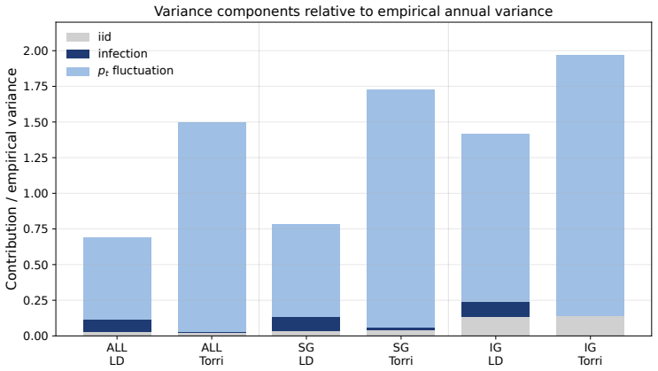
Figure 10 decomposes the empirical variance into contributions from i.i.d
Variance decomposition by subperiod We therefore turn to the variance decomposition, which is central to the present paper. Figure 10 decomposes the empirical variance into contributions from i.i.d. shocks, contagion, and time variation in the default probabilityp t. A clear structural difference emerges across periods. In the early period (1950–1979), th...
-
[13]
R. N. Mantegna and H. E. Stanley,An Introduction to Econophysics: Correlations and Com- plexity in Finance(Cambridge University Press, 1999)
work page 1999
- [14]
- [15]
- [16]
- [17]
- [18]
-
[19]
J. Fernandez-Gracia, K. Suchecki, J. J. Ramasco, M. SanMiguel, and V. M. Egu´ ıluz, Phys. Rev. Lett.112, 158701 (2014)
work page 2014
-
[20]
S. Mori, M. Hisakado, and T. Takahashi, Phys. Rev. E86, 026109 (2012)
work page 2012
-
[21]
S. Mori, K. Nakayama, and M. Hisakado, Phys. Rev. E99, 052307 (2019)
work page 2019
- [22]
-
[23]
P. J. Sch¨ onbucher,Credit Derivatives Pricing Models: Models, Pricing and Implementation (John Wiley & Sons, 2003). 36
work page 2003
-
[24]
S. R. Das, D. Duffie, N. Kapadia, and L. Saita, J. Finance62, 93 (2007)
work page 2007
-
[25]
M. H. A. Davis and V. Lo, Quant. Finance1, 382 (2001)
work page 2001
-
[26]
O. A. Vasicek, KMV Corporation (1991), working paper
work page 1991
-
[27]
O. A. Vasicek, Risk15, 160 (2002)
work page 2002
-
[28]
M. Montagna, G. Torri, and G. Covi,On the Origin of Systemic Risk, Tech. Rep. 2502 (European Central Bank, 2020) ECB Working Paper
work page 2020
- [29]
- [30]
-
[31]
S. Azizpour, K. Giesecke, and G. Schwenkler, J. Financ. Econ.129, 154 (2018)
work page 2018
-
[32]
A. G. Hawkes, Biometrika58, 83 (1971)
work page 1971
- [33]
- [34]
- [35]
-
[36]
de Finetti,Theory of Probability(Wiley, 1974)
B. de Finetti,Theory of Probability(Wiley, 1974). 37
work page 1974
discussion (0)
Sign in with ORCID, Apple, or X to comment. Anyone can read and Pith papers without signing in.