SFUMATO#: A GPU-accelerated code for self-gravitational radiation hydrodynamics simulation with adaptive mesh refinement
Pith reviewed 2026-05-22 10:26 UTC · model grok-4.3
The pith
SFUMATO# implements self-gravitational radiation hydrodynamics on GPUs with adaptive mesh refinement using a linearized chemistry solver.
A machine-rendered reading of the paper's core claim, the machinery that carries it, and where it could break.
Core claim
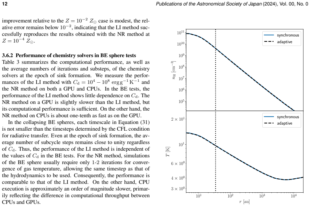
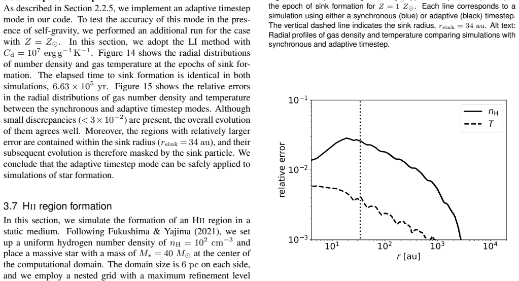
The authors present SFUMATO# as a new implementation that solves self-gravitational radiation hydrodynamics problems using adaptive mesh refinement with the CUDA/HIP programming frameworks. The code includes a multigrid solver for self-gravity, radiation transfer with M1 closure and reduced speed of light, non-equilibrium chemistry, thermal evolution, and sink particles. New solvers based on a linearized implicit method are developed and validated by comparison with Newton-Raphson solutions, and increasing the pseudo dust heat capacity is shown to accelerate the chemistry solver while preserving accuracy up to three orders of magnitude.
What carries the argument
Linearized implicit method for non-equilibrium chemistry and thermal evolution combined with increased pseudo dust heat capacity
If this is right
- The code supports efficient multi-GPU execution via MPI for simulations of giant molecular clouds.
- The self-gravity solver cost grows with the number of MPI processes, so balanced device allocation is required for good scaling.
- Test problems confirm validity of radiation transfer, AMR, and other components alongside the new chemistry solver.
- Accuracy holds for the chemistry and thermal evolution even after the heat capacity adjustment.
Where Pith is reading between the lines
- The boosted heat capacity trick may apply to other astrophysical codes that couple chemistry to hydrodynamics.
- Optimal performance likely requires matching the number of GPUs to the relative costs of gravity and hydro steps.
- Larger domain simulations of star-forming regions become feasible if the scaling behavior generalizes beyond the tested cases.
Load-bearing premise
The linearized implicit method continues to produce accurate solutions even when the pseudo dust heat capacity is increased substantially.
What would settle it
A direct comparison of chemical abundances and temperatures from the chemistry solver on a standard test problem using the realistic dust heat capacity versus the value increased by three orders of magnitude.
Figures


read the original abstract
We present a new implementation of the SFUMATO code, called SFUMATO#, for solving self-gravitational radiation hydrodynamics problems using adaptive mesh refinement (AMR) with the CUDA/HIP programming frameworks. The code incorporates a multigrid solver for self-gravity, radiation transfer with M1 closure and reduced speed of light approximation, non-equilibrium chemistry, thermal evolution, and sink particle schemes. We develop new non-equilibrium chemistry and thermal solvers based on a linearized implicit method, whose accuracy is validated through a series of test problems by comparison with solutions obtained using the Newton-Raphson method. By incorporating the heat capacity of dust grains, the dust temperature can be evolved without iterative energy-balance calculations. From the perspective of computational cost, we demonstrate that adopting an increased pseudo dust heat capacity accelerates the chemistry solver while preserving accuracy, even when the value is increased by up to three orders of magnitude relative to the realistic value. In addition, we perform a suite of test problems to confirm the validity of the other components of our implementation. The code supports multi-GPU execution via MPI-based parallelization. We measure the strong-scaling performance of the hydrodynamics and self-gravity solvers on both uniform and AMR grids, as well as the overall code performance using a giant molecular cloud simulation. We find that the computational cost of the self-gravity solver increases with the number of MPI processes, indicating that efficient parallel performance is achieved only when the number of devices is chosen such that the cost of the self-gravity solver remains comparable to that of the other components.
Editorial analysis
A structured set of objections, weighed in public.
Referee Report
Summary. The manuscript describes SFUMATO#, a new GPU-accelerated implementation of the SFUMATO code for self-gravitational radiation hydrodynamics simulations with adaptive mesh refinement (AMR) using CUDA/HIP. It includes a multigrid self-gravity solver, radiation transfer with M1 closure and reduced speed of light approximation, non-equilibrium chemistry and thermal evolution via a new linearized implicit method (validated against Newton-Raphson), sink particles, and multi-GPU MPI parallelization. Accuracy of the chemistry/thermal solvers is claimed to be preserved even with pseudo dust heat capacity increased by up to three orders of magnitude; strong-scaling performance is measured on uniform/AMR grids and demonstrated in a giant molecular cloud simulation.
Significance. If the validations hold, this provides a practical tool for efficient large-scale simulations of molecular clouds incorporating radiation, chemistry, and self-gravity on GPU architectures. The suite of test problems for component validation and the multi-GPU performance measurements are positive features that support reproducibility and usability.
major comments (1)
- [Abstract (validation of linearized implicit method)] Abstract (validation of linearized implicit method): The central efficiency claim—that increasing the pseudo dust heat capacity by up to three orders of magnitude accelerates the chemistry solver while preserving accuracy—is load-bearing for the new solver's utility. However, no quantitative error metrics (e.g., maximum relative errors in abundances or temperature), specific test conditions (density/temperature/optical depth ranges relevant to molecular clouds), or detailed comparison tolerances versus Newton-Raphson are supplied, leaving unclear whether the approximation remains robust when coupled to radiation transfer and self-gravity.
minor comments (1)
- [Performance measurements] The scaling discussion notes that self-gravity solver cost increases with MPI processes but could be strengthened by explicit tables or figures comparing relative costs of hydrodynamics, gravity, and chemistry components across device counts.
Simulated Author's Rebuttal
We thank the referee for their careful reading and constructive comments on our manuscript. We address the major comment regarding the abstract's description of the linearized implicit solver validation below.
read point-by-point responses
-
Referee: [Abstract (validation of linearized implicit method)] The central efficiency claim—that increasing the pseudo dust heat capacity by up to three orders of magnitude accelerates the chemistry solver while preserving accuracy—is load-bearing for the new solver's utility. However, no quantitative error metrics (e.g., maximum relative errors in abundances or temperature), specific test conditions (density/temperature/optical depth ranges relevant to molecular clouds), or detailed comparison tolerances versus Newton-Raphson are supplied, leaving unclear whether the approximation remains robust when coupled to radiation transfer and self-gravity.
Authors: We agree that the abstract would be clearer with explicit quantitative support for the efficiency claim. The main text already presents detailed comparisons of the linearized implicit method against Newton-Raphson solutions, including maximum relative errors in chemical abundances and gas/dust temperatures across density and temperature ranges relevant to molecular clouds, as well as the specific tolerances used. These validations are performed within the context of the radiation hydrodynamics framework. To address the concern directly, we will revise the abstract to include a concise statement summarizing the quantitative error levels and test conditions. The robustness under coupling is further supported by the full giant molecular cloud simulation, which incorporates radiation transfer, self-gravity, and the chemistry solver simultaneously. revision: yes
Circularity Check
Software implementation and validation paper exhibits no circularity in derivation chain
full rationale
This is a code development and performance paper describing the SFUMATO# implementation for self-gravitational radiation hydrodynamics with AMR, CUDA/HIP, multigrid gravity, M1 radiation, and new linearized implicit chemistry/thermal solvers. The central claims rest on direct comparisons of the new solvers to Newton-Raphson solutions on test problems and on measured scaling in a giant molecular cloud run; these are external benchmarks rather than quantities derived from the same fitted inputs. No equations reduce by construction to prior results, no parameters are fitted to data then relabeled as predictions, and no uniqueness theorems or ansatzes are smuggled via self-citation. Prior SFUMATO references establish code lineage but do not carry the load for the accuracy or performance assertions, which are independently tested. The paper is therefore self-contained against external test benchmarks.
Axiom & Free-Parameter Ledger
free parameters (1)
- pseudo dust heat capacity multiplier =
up to 1000
axioms (2)
- domain assumption M1 closure for radiation transfer
- domain assumption reduced speed of light approximation
Reference graph
Works this paper leans on
-
[1]
Abel, T., Anninos, P., Zhang, Y ., & Norman, M. L. 1997, New Astronomy, Publications of the Astronomical Society of Japan(2024), Vol. 00, No. 021 2, 181
work page 1997
-
[2]
Bakes, E. L. O., & Tielens, A. G. G. M. 1994, ApJ, 427, 822
work page 1994
-
[3]
Berger, M. J., & Colella, P. 1989, Journal of Computational Physics, 82, 64
work page 1989
-
[4]
Berger, M. J., & Oliger, J. 1984, Journal of Computational Physics, 53, 484
work page 1984
-
[5]
Bloch, H., Tremblin, P., González, M., Padioleau, T., & Audit, E. 2021, A&A, 646, A123
work page 2021
- [6]
-
[7]
Diaz-Miller, R. I., Franco, J., & Shore, S. N. 1998, ApJ, 501, 192
work page 1998
-
[8]
Draine, B. T. 2011, Physics of the Interstellar and Intergalactic Medium (Princeton: Princeton University Press)
work page 2011
-
[9]
Federrath, C., Banerjee, R., Clark, P. C., & Klessen, R. S. 2010, ApJ, 713, 269
work page 2010
-
[10]
Ferland, G. J., Peterson, B. M., Horne, K., Welsh, W. F., & Nahar, S. N. 1992, ApJ, 387, 95
work page 1992
-
[11]
Forrey, R. C. 2013, ApJL, 773, L25
work page 2013
- [12]
-
[13]
Fukushima, H., Hosokawa, T., Chiaki, G., et al. 2020, MNRAS, 497, 829
work page 2020
-
[14]
Fukushima, H., Omukai, K., & Hosokawa, T. 2018, MNRAS, 473, 4754
work page 2018
-
[15]
Fukushima, H., & Yajima, H. 2021, MNRAS, 506, 5512 —. 2022, MNRAS, 511, 3346 —. 2023, MNRAS, 524, 1422
work page 2021
- [16]
- [17]
-
[18]
Glover, S. C. O., & Jappsen, A. K. 2007, ApJ, 666, 1
work page 2007
- [19]
- [20]
-
[21]
Hainich, R., Ramachandran, V ., Shenar, T., et al. 2019, A&A, 621, A85
work page 2019
- [22]
-
[23]
He, C.-C., Wibking, B. D., & Krumholz, M. R. 2024, MNRAS, 531, 1228
work page 2024
-
[24]
1990, Numerical computation of internal and external flows
Hirsch, C. 1990, Numerical computation of internal and external flows. V ol. 2 (New York: John Wiley & Sons) - Computational methods for inviscid and viscous flows
work page 1990
-
[25]
Hockney, R. W., & Eastwood, J. W. 1981, Computer Simulation Using Particles (New York: McGraw-Hill)
work page 1981
-
[26]
Hollenbach, D., & McKee, C. F. 1979, ApJS, 41, 555
work page 1979
- [27]
- [28]
-
[29]
Inoguchi, M., Hosokawa, T., Mineshige, S., & Kim, J.-G. 2020, MNRAS, 497, 5061
work page 2020
-
[30]
Inutsuka, S.-i., Inoue, T., Iwasaki, K., & Hosokawa, T. 2015, A&A, 580, A49
work page 2015
-
[31]
Kimura, K., Sugimura, K., Hosokawa, T., Fukushima, H., & Omukai, K. 2026, ApJ, 999, 257
work page 2026
-
[32]
Kreckel, H., Bruhns, H., ˇCížek, M., et al. 2010, Science, 329, 69
work page 2010
-
[33]
Krumholz, M. R., Klein, R. I., McKee, C. F., & Bolstad, J. 2007, ApJ, 667, 626
work page 2007
-
[34]
Laor, A., & Draine, B. T. 1993, ApJ, 402, 441
work page 1993
-
[35]
Larson, R. B. 1985, MNRAS, 214, 379 —. 2005, MNRAS, 359, 211
work page 1985
- [36]
- [37]
-
[38]
Levermore, C. D. 1984, J. Quant. Spectrosc. Radiat. Transfer, 31, 149
work page 1984
-
[39]
N., Inutsuka, S.-i., & Matsumoto, T
Machida, M. N., Inutsuka, S.-i., & Matsumoto, T. 2010, ApJ, 724, 1006
work page 2010
- [40]
- [41]
- [42]
- [43]
-
[44]
H., Federrath, C., & Krumholz, M
Menon, S. H., Federrath, C., & Krumholz, M. R. 2022, MNRAS, 517, 1313
work page 2022
-
[45]
Mihalas, D., & Mihalas, B. W. 1984, Foundations of radiation hydrodynam- ics
work page 1984
- [46]
- [47]
-
[48]
Omukai, K., Tsuribe, T., Schneider, R., & Ferrara, A. 2005, ApJ, 626, 627
work page 2005
-
[49]
Osterbrock, D. E. 1989, Astrophysics of gaseous nebulae and active galactic nuclei (Mill Valley: University Science Books)
work page 1989
- [50]
-
[51]
Petrosian, V ., Silk, J., & Field, G. B. 1972, ApJL, 177, L69
work page 1972
-
[52]
Roe, P. L. 1981, Journal of Computational Physics, 43, 357
work page 1981
-
[53]
Rosdahl, J., Blaizot, J., Aubert, D., Stranex, T., & Teyssier, R. 2013, MNRAS, 436, 2188
work page 2013
- [54]
-
[55]
Schive, H.-Y ., ZuHone, J. A., Goldbaum, N. J., et al. 2018, MNRAS, 481, 4815
work page 2018
- [56]
- [57]
- [58]
-
[59]
Stone, J. M., Tomida, K., White, C. J., & Felker, K. G. 2020, ApJS, 249, 4
work page 2020
-
[60]
Stone, J. M., Mullen, P. D., Fielding, D., et al. 2024, arXiv e-prints, arXiv:2409.16053
-
[61]
Sugimura, K., Hosokawa, T., Yajima, H., & Omukai, K. 2017, MNRAS, 469, 62
work page 2017
- [62]
-
[63]
Tielens, A. G. G. M., & Hollenbach, D. 1985, ApJ, 291, 722
work page 1985
-
[64]
Tomida, K., & Stone, J. M. 2023, ApJS, 266, 7
work page 2023
-
[65]
Toro, E. F., Spruce, M., & Speares, W. 1994, Shock waves, 4, 25
work page 1994
- [66]
-
[67]
1984, Journal of Computational Physics, 54, 115
Woodward, P., & Colella, P. 1984, Journal of Computational Physics, 54, 115
work page 1984
-
[68]
Zhang, W., Howell, L., Almgren, A., Burrows, A., & Bell, J. 2011, ApJS, 196, 20 Appendix 1 Chemical network In Table 11, we summarize the chemical network consisting ofH, H2,H +, ande −. The abundance ofH − is obtained as an interme- diate species, following the treatment described in Appendix A of Omukai et al. (2010). The photoionization rate of hydroge...
work page 2011
discussion (0)
Sign in with ORCID, Apple, or X to comment. Anyone can read and Pith papers without signing in.