Delay Modeling with Conformable and Caputo Derivatives: Analytical and Computational Insights
Pith reviewed 2026-05-08 10:23 UTC · model grok-4.3
The pith
Conformable derivatives deliver stable analytic-numerical agreement for fractional delay equations while Caputo versions accumulate long-term discretization errors.
A machine-rendered reading of the paper's core claim, the machinery that carries it, and where it could break.
Core claim
For fractional-order delay differential equations the conformable derivative admits an associated Laplace transform that keeps the algebraic structure intact, allowing explicit solutions via series expansions of the delay terms; the resulting analytic expressions agree with basic Euler and Runge-Kutta integrations over long intervals, while the Caputo derivative's memory kernel forces the use of higher-order or series-anchored schemes to suppress accumulating discretization noise and maintain accuracy.
What carries the argument
The conformable Laplace transform together with series expansions of the delay argument, which together convert the fractional delay equation into an algebraic problem whose solutions remain causal and finite.
If this is right
- Explicit solutions become available for a range of conformable delay models without resorting to numerical approximation from the outset.
- Basic first-order integrators suffice to maintain long-term accuracy in conformable cases, reducing the need for specialized high-order codes.
- Caputo-based delay models can be made reliable only by anchoring the scheme to a series expansion or by increasing the order of the discretization.
- The conformable approach supplies a direct physical interpretation for the fractional order and the delay, unlike memory-integral formulations.
Where Pith is reading between the lines
- The same conformable Laplace machinery could be applied to systems with state-dependent or distributed delays common in biology and control.
- Switching from Caputo to conformable might simplify real-time simulation of delayed fractional systems in engineering hardware.
- Comparative tests on experimental time-series data with known delays would reveal whether the conformable solutions better match observed transients.
Load-bearing premise
That the series expansions used to incorporate delay terms inside the conformable Laplace framework preserve causality and do not generate unphysical artifacts or lose interpretability.
What would settle it
Integrate a simple linear conformable delay equation whose closed-form solution is known, using only the basic Euler method over a long time horizon, and check whether the numerical trajectory remains within a small, non-growing error bound of the analytic solution.
Figures


read the original abstract
This work presents an analytical and computational study of fractional-order delay differential equations formulated using both the conformable and Caputo derivatives. For the conformable case, we develop the associated integral, exponential function, and Laplace transform, showing how the conformable Laplace framework preserves algebraic structure and facilitates explicit solutions. Delay terms are treated through series expansions and transform-based methods, ensuring causal and finite representations. In parallel, Caputo-based formulations are examined, highlighting the challenges posed by convolutional memory kernels and the potential for long-term numerical instability. Numerical implementations are carried out using mesh-aligned algorithms: Euler and Runge--Kutta schemes for conformable dynamics, and Euler, L2--$\sigma$, and a series--anchored predictor--corrector method for Caputo dynamics. Comparative experiments demonstrate that conformable derivatives yield stable, consistent agreement between analytic and numerical solutions, whereas Caputo dynamics require higher-order or series-anchored schemes to suppress discretization noise and maintain long-term accuracy. These results underscore the advantages of the conformable formalism in modeling dynamic phenomena with delay and memory, offering a tractable and physically interpretable alternative to integral-based fractional models.
Editorial analysis
A structured set of objections, weighed in public.
Referee Report
Summary. This manuscript investigates fractional delay differential equations using both conformable and Caputo fractional derivatives. Analytically, it derives the integral operator, exponential function, and Laplace transform for the conformable derivative, employing series expansions and transform methods to incorporate delay terms while maintaining causality. For the Caputo derivative, it addresses the difficulties arising from the memory kernel. Computationally, it implements Euler and Runge-Kutta methods for conformable equations and compares them to Euler, L2-σ, and a series-anchored predictor-corrector scheme for Caputo equations. The key finding is that conformable formulations achieve stable and consistent analytic-numerical agreement using standard integrators, whereas Caputo formulations exhibit discretization noise unless higher-order or specialized schemes are used, suggesting conformable derivatives as a more tractable modeling choice for delayed systems.
Significance. If the reported numerical advantages are confirmed to stem from the properties of the conformable derivative rather than differences in discretization schemes, the work would offer a valuable alternative framework for fractional delay models that avoids the computational overhead of non-local operators. The analytical tools developed for conformable derivatives with delays could enable closed-form solutions in certain cases and facilitate easier numerical implementation. This could be significant in applied mathematics and modeling of systems with memory and delay, such as in biology or control theory, provided the comparisons are made rigorous.
major comments (2)
- [Numerical implementations and comparative experiments] Numerical implementations (as described in the abstract): the experiments apply Euler and Runge-Kutta schemes to conformable dynamics but L2-σ and series-anchored predictor-corrector methods to Caputo dynamics. This does not hold the discretization scheme fixed, so the claimed stability and accuracy advantages of conformable derivatives cannot be unambiguously attributed to the derivative type rather than the choice of integrator; a controlled comparison using the same scheme on both is required to support the central claim that conformable is a 'tractable alternative'.
- [Comparative experiments] The manuscript provides no specific parameter values for the delay equations, time intervals, error metrics (e.g., L2 or maximum error), or quantitative bounds on the 'consistent agreement' and 'discretization noise' reported in the experiments. This absence makes the comparative results qualitative and prevents independent verification of the headline performance gap.
minor comments (2)
- [Numerical implementations] The term 'mesh-aligned algorithms' is introduced without definition or reference, which may obscure the numerical methodology for readers.
- [Abstract] The abstract would be strengthened by naming the specific delay differential equation examples (e.g., the form of the test problems) used to generate the reported agreement between analytic and numerical solutions.
Simulated Author's Rebuttal
We thank the referee for the careful reading and constructive comments on our manuscript. The suggestions highlight important aspects of making the numerical comparisons more rigorous, and we will revise the paper to address them directly.
read point-by-point responses
-
Referee: Numerical implementations (as described in the abstract): the experiments apply Euler and Runge-Kutta schemes to conformable dynamics but L2-σ and series-anchored predictor-corrector methods to Caputo dynamics. This does not hold the discretization scheme fixed, so the claimed stability and accuracy advantages of conformable derivatives cannot be unambiguously attributed to the derivative type rather than the choice of integrator; a controlled comparison using the same scheme on both is required to support the central claim that conformable is a 'tractable alternative'.
Authors: We agree that the current setup uses schemes tailored to each derivative type, which prevents isolating the effect of the derivative alone. To address this, we will add a controlled comparison in the revised manuscript by applying the same Euler method to both conformable and Caputo delay equations under identical parameters and time intervals. This will allow direct attribution of any observed differences to the derivative formulation while retaining the original results (which demonstrate that Caputo requires specialized schemes for stability) as supplementary evidence of practical tractability. revision: yes
-
Referee: The manuscript provides no specific parameter values for the delay equations, time intervals, error metrics (e.g., L2 or maximum error), or quantitative bounds on the 'consistent agreement' and 'discretization noise' reported in the experiments. This absence makes the comparative results qualitative and prevents independent verification of the headline performance gap.
Authors: We accept this criticism; the absence of explicit parameters and metrics renders the comparisons insufficiently quantitative. In the revision, we will specify all parameters (e.g., delay value τ, fractional order α, initial conditions, and integration interval [0,T]), report L2 and maximum absolute errors for each method, and include tables or figures with quantitative bounds on agreement and noise levels. This will enable independent verification and strengthen the central claims. revision: yes
Circularity Check
No load-bearing circularity; minor self-citations only
full rationale
The paper's derivation chain consists of explicit constructions of the conformable integral, exponential, and Laplace transform from the standard conformable derivative definition, followed by series expansions for delay terms and direct numerical comparisons using stated schemes. These steps are self-contained and do not reduce to fitted parameters, self-referential definitions, or unverified self-citations. The central comparative claim rests on the reported experiments rather than any tautological renaming or imported uniqueness theorem. Any self-citations to prior conformable work are peripheral and not load-bearing for the delay-modeling results or stability conclusions.
Axiom & Free-Parameter Ledger
axioms (2)
- standard math Standard algebraic properties of the conformable derivative, including existence of integral, exponential function, and Laplace transform that preserve structure
- domain assumption Delay terms admit causal and finite representations via series expansions and transform methods
Reference graph
Works this paper leans on
-
[1]
the geometric factorae −sT α/α/sis uniformly small on the chosen inversion con- tour
-
[2]
24 These hypotheses are standard in transform methods and should be verified in concrete applications
termwise differentiation and integration under the integral sign are justified by dominated convergence. 24 These hypotheses are standard in transform methods and should be verified in concrete applications. When the above analytic conditions hold, the conformable transform route yields explicit, finite (for fixedt) series solutions obtained by straightfo...
-
[3]
Laplace-domain representation For the analysis, we require L ( tα α k) (s),(111) and since tα α k = tαk αk ,L{t ν}(s) = Γ(ν+ 1) sν+1 , ν >−1,(112) we obtain L ( tα α k) (s) = 1 αk Γ(αk+ 1) sαk+1 .(113) This identity will be used repeatedly, since each term contributes a rational power ofs weighted by Gamma-function coefficients. 25 Applying the Laplace tr...
-
[4]
This is because the Caputo derivative introduces a memory kernel that weights past values with a decaying fractional power
Long term behavior for constant forcingb(t) =b 0 When the external inputb(t) =b 0 is constant, the effect of the delay term becomes asymptotically negligible in the Caputo framework. This is because the Caputo derivative introduces a memory kernel that weights past values with a decaying fractional power. For long times, the contribution of delayed states...
-
[5]
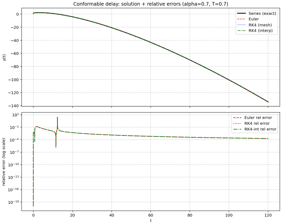
Example 1 The numerical performance of the three schemes is evaluated under the parameter set α= 0.7,a= 0.5,T= 0.7,y 0 = 1.0,h= 0.001, andb coeffs = [1.0,0.2,−0.05]. The corresponding numerical trajectories and their relative errors with respect to the analytical series solutions are shown in Figure 1, providing a direct visual comparison of accuracy and ...
-
[6]
Example 2 The numerical performance of the three schemes is evaluated for the parameter setα= 0.7,a= 0.5,T= 2,y 0 = 1.0,h= 0.001, andb coeffs = [1.0,0.2,−0.05]. Figure 2 presents the resulting numerical trajectories together with their relative errors with respect to the analytical series solution, allowing a direct visual assessment of accuracy across th...
-
[7]
Example 3 The numerical performance of the three schemes is evaluated for the parameter set α= 0.7,a= 0.5,T= 3,y 0 = 1.0,h= 0.001, andb coeffs = [1.0,0.2,−0.05]. Figure 3 displays the resulting numerical trajectories together with their relative errors with respect to the analytical series solution, providing a direct visual assessment of the accuracy of ...
-
[8]
Example 4 The numerical performance of the three schemes is evaluated for the parameter setα= 0.7,a= 0.5,T= 5,y 0 = 1.0,h= 0.001, andb coeffs = [1.0,0.2,−0.05]. Figure 4 presents the resulting numerical trajectories together with their relative errors with respect to the analytical series solution, offering a direct visual assessment of the accuracy of ea...
-
[9]
Example 5 The numerical performance of the three schemes is evaluated for the parameter set α= 0.7,a= 1.1,T= 3,y 0 = 1.0,h= 0.001, andb coeffs = [1.0,0.2,−0.05]. Figure 5 shows the resulting numerical trajectories together with their relative errors with respect to the analytical series solution, providing a direct visual assessment of the accuracy of eac...
-
[10]
Thepredictorevaluates the truncated analytic series att n+1, providing an anchor consistent with the exact solution structure
-
[11]
Thecorrectorapplies a fractional Adams–Moulton step: ycorr n+1 =y n + hα Γ(α+ 1) 1 2 fn + 1 2 fn+1 ,(171) wheref n =b(t n)−a y(t n −T) andf n+1 =b(t n+1)−a y(t n+1 −T)
-
[12]
Error analysis.The analytic truncated series serves as a reference solution
Ablending stepaverages predictor and corrector values: yn+1 = 1 2 ycorr n+1 + 1 2 ypred n+1 ,(172) improving stability and reducing oscillations. Error analysis.The analytic truncated series serves as a reference solution. The abso- lute error is defined as Eabs(tn) =|y num n −y series n |,(173) and the relative error as Erel(tn) = Eabs(tn) |yseries n |+ ...
2024
-
[13]
Then: TαF(t) =t 1−α d dt Z t 0 τ α−1f(τ)dτ =f(t).(A11) 69
Conformable Integral as Inverse Operator The conformable integral of orderα∈(0,1] is defined as: Iαf(t) := Z t 0 τ α−1f(τ)dτ.(A9) This integral acts as the inverse ofT α in the following sense: Tα[Iαf(t)] =f(t).(A10) Proof.LetF(t) =I αf(t) = R t 0 τ α−1f(τ)dτ. Then: TαF(t) =t 1−α d dt Z t 0 τ α−1f(τ)dτ =f(t).(A11) 69
-
[14]
Let 0< α≤1 and suppose that the conformable Laplace transform is defined by: Lα[f(t)](s) = Z ∞ 0 e− stα α f(t)t α−1dt.(A16) Proof.1
Conformable Laplace Transform The conformable Laplace transform of a functionf: [0,∞)→Ris given by: Lα{f(t)}(s) := Z ∞ 0 f(t)e −stα/αtα−1 dt.(A12) Iffis differentiable andf(0) is well defined, then: Lα{Tαf(t)}(s) =sL α{f(t)}(s)−f(0).(A13) Proof.SinceT αf(t) =t 1−αf ′(t), we compute: Lα{Tαf(t)}(s) = Z ∞ 0 f ′(t)e−stα/α dt.(A14) Using classical integration ...
-
[15]
Forf(t) =t q, whereq∈R: Lα[tq](s) = Z ∞ 0 e− stα α tq tα−1dt= Z ∞ 0 tq+α−1e− stα α dt.(A21) Using the same change of variable as in item 1: u= stα α , t= αu s 1/α , dt= α s 1/α · 1 α u 1 α −1du.(A22) Substituting into the integral: Lα[tq](s) = Z ∞ 0 αu s q+α−1 α e−u α s 1/α · 1 α u 1 α −1du(A23) = α s q+α α · 1 α Z ∞ 0 u q α e−udu(A24) =α q/αs−(1+q/α)Γ 1 ...
-
[16]
Conformable Laplace Transform of a Delayed Function Iff(t) = 0 fort <0, andT >0, then: Lα{f(t−T)}(s) =e −sT α/α · Lα{f(t)}(s).(A26) This mirrors the classical case, where temporal delays appear as exponential multiplica- tive factors in the Laplace domain
-
[17]
Fractional derivative quantum fields at positive temperature.Phys
Lim, S.C. Fractional derivative quantum fields at positive temperature.Phys. A2006, 363, 269–281.https://doi.org/10.1016/j.physa.2005.08.005
-
[18]
Fractional derivatives generalization of Einstein‘s field equations.Indian J
El-Nabulsi, A.R. Fractional derivatives generalization of Einstein‘s field equations.Indian J. Phys.2013,87, 195–200.https://doi.org/10.1007/s12648-012-0201-4
-
[19]
Fractional Dynamics from Einstein Gravity, General Solutions, and Black Holes
Vacaru, S.I. Fractional Dynamics from Einstein Gravity, General Solutions, and Black Holes. Int. J. Theor. Phys.2012,51, 1338–1359.https://doi.org/10.1007/s10773-011-1010-9
-
[20]
Moniz, P.V.; Jalalzadeh, S. From Fractional Quantum Mechanics to Quantum Cosmology: An Overture.Mathematics2020,8, 313.https://doi.org/10.3390/math8030313. 71
-
[21]
Cosmology under the fractional calculus approach.Mon
Garc´ ıa-Aspeitia, M.A.; Fernandez-Anaya, G.; Hern´ andez-Almada, A.; Leon, G.; Maga˜ na, J. Cosmology under the fractional calculus approach.Mon. Not. Roy. Astron. Soc.2022, 517, 4813–4826.https://doi.org/10.1093/mnras/stac3006
-
[22]
Exact solutions and cosmological con- straints in fractional cosmology.Fractal Fract.2023,7, 368.https://doi.org/10.3390/ fractalfract7050368
Gonz´ alez, E.; Leon, G.; Fernandez-Anaya, G. Exact solutions and cosmological con- straints in fractional cosmology.Fractal Fract.2023,7, 368.https://doi.org/10.3390/ fractalfract7050368
2023
-
[23]
Leon Torres, G.; Garc´ ıa-Aspeitia, M.A.; Fernandez-Anaya, G.; Hern´ andez-Almada, A.; Maga˜ na, J.; Gonz´ alez, E. Cosmology under the fractional calculus approach: A possibleH 0 tension resolution?PoS2023,CORFU2022, 248.https://doi.org/10.22323/1.436.0248
-
[24]
Revisit- ing Fractional Cosmology.Fractal Fract.2023,7, 149.https://doi.org/10.3390/ fractalfract7020149
Micolta-Riascos, B.; Millano, A.D.; Leon, G.; Erices, C.; Paliathanasis, A. Revisit- ing Fractional Cosmology.Fractal Fract.2023,7, 149.https://doi.org/10.3390/ fractalfract7020149
2023
-
[25]
El-Nabulsi, R.A. Nonlocal-in-time kinetic energy in nonconservative fractional systems, disor- dered dynamics, jerk and snap and oscillatory motions in the rotating fluid tube.Int. J.-Non- Linear Mech.2017,93, 65–81.https://doi.org/10.1016/j.ijnonlinmec.2017.04.010
-
[26]
Barrientos, E.; Mendoza, S.; Padilla, P. Extending Friedmann equations using fractional derivatives using a Last Step Modification technique: The case of a matter dominated accelerated expanding Universe.Symmetry2021,13, 174.https://doi.org/10.3390/ sym13020174
-
[27]
Fractional Action-Like Variational Problems
El-Nabulsi, R.A.; Torres, D.F. Fractional Action-Like Variational Problems. J. Math. Phys. 2008, 49, 053521
2008
-
[28]
Fractional Scalar Field Cosmology.Fractal Fract
Rasouli, S.M.M.; Cheraghchi, S.; Moniz, P. Fractional Scalar Field Cosmology.Fractal Fract. 2024,8, 281.https://doi.org/10.3390/fractalfract8050281
-
[29]
K. Marroqu´ ın, G. Leon, A. D. Millano, C. Michea and A. Paliathanasis, Conformal and Non- Minimal Couplings in Fractional Cosmology, Fractal Fract.8(2024), 253https://doi.org/ 10.3390/fractalfract8050253
-
[30]
B. Micolta-Riascos, A. D. Millano, G. Leon, B. Droguett, E. Gonz´ alez and J. Maga˜ na, Frac- tional Einstein-Gauss-Bonnet scalar field cosmology, Fractal Fract.8(2024), 626https: //doi.org/10.3390/fractalfract8110626
-
[31]
Micolta-Riascos, B., Droguett, B., Mattar Marriaga, G., Leon, G., Paliathanasis, A., del Campo, L., & Leyva, Y. (2025). Fractional Time-Delayed Differential Equations: Applica- 72 tions in Cosmological Studies. Fractal and Fractional, 9(5), 318.https://doi.org/10.3390/ fractalfract9050318
2025
-
[32]
A New Definition of Fractional Derivative
Khalil, R.; Al Horani, M.; Yousef, A.; Sababheh, M. A New Definition of Fractional Derivative. J. Comput. Appl. Math.2014,264, 65–70.https://doi.org/10.1016/j.cam.2014.01.002
-
[33]
Bounded and periodic solutions in retarded difference equations using summable dichotomies.Dyn
Del Campo, L.; Pinto, M.; Vidal, C. Bounded and periodic solutions in retarded difference equations using summable dichotomies.Dyn. Syst. Appl.2012,21, 1
2012
-
[34]
Bounded and periodic solutions for abstract functional difference equations with summable dichotomies: Applications to Volterra systems.Bull
Del Campo, L.; Pinto, M.; Vidal, C. Bounded and periodic solutions for abstract functional difference equations with summable dichotomies: Applications to Volterra systems.Bull. Math. Soc. Sci. Math. Roum.2018,61, 279–292
2018
-
[35]
Almost and asymptotically almost periodic solutions of abstract retarded functional difference equations in phase space.J
Del Campo, L.; Pinto, M.; Vidal, C. Almost and asymptotically almost periodic solutions of abstract retarded functional difference equations in phase space.J. Differ. Equ. Appl.2011, 17, 915–934
2011
-
[36]
Weighted exponential trichotomy of difference equations and asymptotic behavior for nonlinear systems.Dyn
Cuevas, C.; del Campo, L.; Vidal, C. Weighted exponential trichotomy of difference equations and asymptotic behavior for nonlinear systems.Dyn. Contin. Discrete Impuls. Syst. Ser. A Math. Anal.2010,17, 377–400
2010
-
[37]
Weighted exponential trichotomy of difference equations
Vidal, C.; Cuevas, C.; del Campo, L. Weighted exponential trichotomy of difference equations. Dyn. Syst. Appl.2008,5, 489–495
2008
-
[38]
Asymptotic expansion for difference equations with infinite delay
Cuevas, C.; del Campo, L. Asymptotic expansion for difference equations with infinite delay. Asian-Eur. J. Math.2009,2, 19–40
2009
-
[39]
Existence and stability of solution for time-delayed nonlinear fractional differential equations.Appl
Geremew Kebede, S.; Guezane Lakoud, A. Existence and stability of solution for time-delayed nonlinear fractional differential equations.Appl. Math. Sci. Eng.2024,32, 2314649
2024
-
[40]
A class of Langevin time-delay differential equations with general fractional orders and their applications to vibration theory.J
Huseynov, I.T.; Mahmudov, N.I. A class of Langevin time-delay differential equations with general fractional orders and their applications to vibration theory.J. King Saud Univ.-Sci. 2021,33, 101596
2021
-
[41]
A numerical method based on finite difference for solving fractional delay differential equations.J
Moghaddam, B.P.; Mostaghim, Z.S. A numerical method based on finite difference for solving fractional delay differential equations.J. Taibah Univ. Sci.2013,7, 120–127
2013
-
[42]
Numerical solution of multi-order fractional differential equations with multiple delays via spectral collocation methods.Appl
Dabiri, A.; Butcher, E.A. Numerical solution of multi-order fractional differential equations with multiple delays via spectral collocation methods.Appl. Math. Model.2018,56, 424–448
2018
-
[43]
A computational algorithm for the numerical solution of fractional order delay differential equations.Appl
Amin, R.; Shah, K.; Asif, M.; Khan, I. A computational algorithm for the numerical solution of fractional order delay differential equations.Appl. Math. Comput.2021,402, 125863
2021
-
[44]
Opti- 73 mal control of nonlinear time-delay fractional differential equations with Dickson polynomials
Chen, S.B.; Soradi-Zeid, S.; Alipour, M.; Chu, Y.M.; Gomez-Aguilar, J.; Jahanshahi, H. Opti- 73 mal control of nonlinear time-delay fractional differential equations with Dickson polynomials. Fractals2021,29, 2150079
-
[45]
Stability and stabilization of fractional order time delay systems.Sci
Lazarevi´ c, M. Stability and stabilization of fractional order time delay systems.Sci. Tech. Rev.2011,61, 31–45
2011
-
[46]
Stability analysis of time-delayed linear fractional- order systems.Int
Pakzad, M.A.; Pakzad, S.; Nekoui, M.A. Stability analysis of time-delayed linear fractional- order systems.Int. J. Control. Autom. Syst.2013,11, 519–525
2013
-
[47]
Luo, A.C.; Sun, J.Q.Complex Systems: Fractionality, Time-Delay and Synchronization; Springer Science & Business Media: Berlin/Heidelberg, Germany, 2011
2011
-
[48]
Fractional derivative and time delay damper characteristics in Duffing–van der Pol oscillators.Commun
Leung, A.Y.; Guo, Z.; Yang, H. Fractional derivative and time delay damper characteristics in Duffing–van der Pol oscillators.Commun. Nonlinear Sci. Numer. Simul.2013,18, 2900–2915
2013
-
[49]
The stability and control of fractional nonlinear system with distributed time delay.Appl
Hu, J.B.; Zhao, L.D.; Lu, G.P.; Zhang, S.B. The stability and control of fractional nonlinear system with distributed time delay.Appl. Math. Model.2016,40, 3257–3263
2016
-
[50]
Mathai, A.M.; Haubold, H.J.Special Functions for Applied Scientists; Springer: Berlin/Hei- delberg, Germany, 2008
2008
-
[51]
The special functions of fractional calculus as generalized fractional calculus operators of some basic functions.Comput
Kiryakova, V. The special functions of fractional calculus as generalized fractional calculus operators of some basic functions.Comput. Math. Appl.2010,59, 1128–1141
2010
-
[52]
Yang, X.J.Theory and Applications of Special Functions for Scientists and Engineers; Springer: Berlin/Heidelberg, Germany, 2021
2021
-
[53]
Agarwal, P.; Agarwal, R.P.; Ruzhansky, M.Special Functions and Analysis of Differential Equations; CRC Press: Boca Raton, FL, USA, 2020
2020
-
[54]
Abdeljawad, T. On Conformable Calculus.J. Comput. Appl. Math.2015,279, 57–66.https: //doi.org/10.1016/j.cam.2014.10.016
-
[55]
Introduction to Functional Differential Equations,
J. K. Hale and S. M. Verduyn Lunel, “Introduction to Functional Differential Equations,”Applied Mathematical Sciences, vol. 99, Springer, Dordrecht, 1993. DOI:10.1007/978-1-4612-4342-7.https://link.springer.com/book/10.1007/ 978-1-4612-4342-7
work page doi:10.1007/978-1-4612-4342-7.https://link.springer.com/book/10.1007/ 1993
-
[56]
Delay Differential Equations in Single Species Dynamics,
S. Ruan, “Delay Differential Equations in Single Species Dynamics,” inDelay Differential Equations and Applications, O. Arino, M. L. Hbid, and E. Ait Dads, Eds., NATO Sci- ence Series II: Mathematics, Physics and Chemistry, vol. 205, Springer, Dordrecht, 2006, pp. 477–517. DOI:10.1007/1-4020-3647-7 11.https://link.springer.com/chapter/10. 1007/1-4020-3647-7_11 74
-
[57]
Delay Differential Equations and Applica- tions,
O. Arino, M. L. Hbid, and E. Ait Dads, Eds., “Delay Differential Equations and Applica- tions,” NATO Science Series II: Mathematics, Physics and Chemistry, vol. 205, Springer, Dor- drecht, 2006. DOI:10.1007/1-4020-3647-7.https://link.springer.com/book/10.1007/ 1-4020-3647-7
work page doi:10.1007/1-4020-3647-7.https://link.springer.com/book/10.1007/ 2006
-
[58]
Stability Analysis of Linear Conformable Differential Equations System with Time Delays.Adv
Mohammadnezhad, V.; Eslami, M.; Rezazadeh, H. Stability Analysis of Linear Conformable Differential Equations System with Time Delays.Adv. Differ. Equ.2022,2022, 1–16.https: //doi.org/10.5269/bspm.v38i6.37010
-
[59]
Prakash, A.; Goyal, M.; Gupta, S. Fractional variational iteration method for solving time- fractional Newell–Whitehead–Segel equation.Nonlinear Engineering,2019,8(1), 164–171. https://doi.org/10.1515/nleng-2018-0001
-
[60]
A Computational Approach to Exponential-Type Variable-Order Fractional Differential Equations
Garrappa, R.; Giusti, A. A Computational Approach to Exponential-Type Variable-Order Fractional Differential Equations. J. Sci. Comput. 2023, 96, 63.https://doi.org/10.1007/ s10915-023-02283-6
2023
- [61]
-
[62]
A., Vald´ es, R., Quezada-T´ ellez, L
Fern´ andez-Anaya, G., God´ ınez, F. A., Vald´ es, R., Quezada-T´ ellez, L. A., & Polo-Labarrios, M. A. (2025). A Simple Fractional Model with Unusual Dynamics in the Derivative Order. Fractal and Fractional, 9(4), 264.https://doi.org/10.3390/fractalfract9040264
-
[63]
On a discrete composition of the fractional integral and Caputo derivative,
L. P lociniczak, “On a discrete composition of the fractional integral and Caputo derivative,” Communications in Nonlinear Science and Numerical Simulation, vol. 108, p. 106234, 2022. doi: 10.1016/j.cnsns.2021.106234
-
[64]
Fractional Euler method; an effective tool for solving fractional differential equations,
H. F. Ahmed, “Fractional Euler method; an effective tool for solving fractional differential equations,”Journal of the Egyptian Mathematical Society, vol. 26, no. 1, 2018. 75
2018
discussion (0)
Sign in with ORCID, Apple, or X to comment. Anyone can read and Pith papers without signing in.