The Tracking Tapered Gridded Estimator for the 21-cm power spectrum from the Murchison Widefield Array (MWA) drift scan observations -- III. Improved upper limits at z = 8.2 from multiple pointings
Pith reviewed 2026-05-08 01:53 UTC · model grok-4.3
The pith
Incoherently combining 23 MWA pointings produces the tightest upper limit yet on the 21-cm power spectrum at redshift 8.2 from this telescope.
A machine-rendered reading of the paper's core claim, the machinery that carries it, and where it could break.
Core claim
The authors show that the range 358.5° ≤ α ≤ 11.5° contains 23 pointing centers whose measured power is consistent with noise; incoherently combining these centers gives the 2σ upper limit Δ_UL²(k) = (98.67)^2 mK² at k = 0.156 Mpc^{-1} for the 21-cm signal at z = 8.2, the lowest value obtained with the MWA at this epoch.
What carries the argument
The Tracking Tapered Gridded Estimator (TTGE) applied to multiple drift-scan pointing centers, together with angular power spectrum D_ℓ(α) to flag and exclude regions contaminated by Fornax A.
If this is right
- The new limit is approximately two times higher than existing LOFAR bounds and twenty-one times higher than HERA bounds at comparable redshifts.
- The measured upper limit lies roughly three orders of magnitude above theoretical predictions for the 21-cm signal during reionization.
- The single best pointing center alone gives a 2σ limit of (173.13)^2 mK² at k = 0.161 Mpc^{-1}, showing that the combination step provides the main improvement.
- The strategy of mapping D_ℓ versus right ascension and retaining only the cleanest pointings can be repeated on larger MWA datasets to push the bound lower.
Where Pith is reading between the lines
- The same foreground-avoidance and multi-pointing averaging approach could be tested on other low-frequency arrays to check whether comparable gains appear.
- If faint diffuse foregrounds remain below current detection thresholds in the selected regions, the true cosmological limit would be weaker than reported, motivating cross-validation with independent pipelines.
- Extending the clean range beyond the current 23 pointings would require either more data or refined sidelobe modeling of sources like Fornax A.
Load-bearing premise
The selected 23 pointings contain no residual foreground power or unaccounted systematics beyond the identified Fornax A peaks, so that all measured power is instrumental noise.
What would settle it
An independent deeper integration or cross-check analysis that detects excess power above the noise floor in the same selected pointings, or that measures a 21-cm signal amplitude below 98.67 mK at k ≈ 0.156 Mpc^{-1}.
Figures


read the original abstract
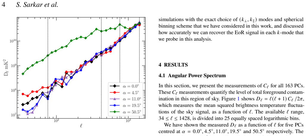
We analyze zenith-pointing $(\delta=-26.7^{\circ})$ Murchison Widefield Array (MWA) $\nu_c=154.2 \,{\rm MHz}$ drift scan observations covering $349.0^{\circ} \le \alpha \le 70.0^{\circ}$ with 163 pointing centers (PCs) spaced by $0.5^{\circ}$. We measure $D_{\ell}$, the mean-squared angular brightness temperature fluctuations, as a function of $\alpha$. A broad peak at $\alpha \approx 50.0^{\circ}$ corresponds to the bright extended source Fornax~A in the main lobe of the primary beam. A smaller peak at $\alpha \approx 5.0^{\circ}$ possibly corresponds to Fornax~A in the first sidelobe. For $\alpha \leq 22.0^{\circ}$ and $\ell \ge 200$, we find $D_{\ell} \propto \ell^2$, which we interpret as Poisson fluctuations from point sources. We present $\Delta^2(k)$, the mean-squared 21-cm brightness temperature fluctuations from the Epoch of Reionization, as a function of $\alpha$. Fornax~A causes strong contamination near $\alpha \approx 50.5^{\circ}$, elsewhere several PCs are consistent with noise. The range $358.5^{\circ} \leq \alpha \leq 11.5^{\circ}$ is relatively foreground-free and best suited for EoR science. The PC at $\alpha = 11.0^{\circ}$ yields the best $2\sigma$ upper limit $\Delta^{2}_{\rm UL}(k) = (173.13)^{2}\,{\rm mK^{2}}$ at $k = 0.161\,{\rm Mpc^{-1}}$. We incoherently combine $23$ PCs to obtain $\Delta_{\rm UL}^2(k)=(98.67)^{2}\,{\rm mK}^{2}$ at $k=0.156\,{\rm Mpc}^{-1}$. This is the tightest upper limit from the MWA, being $\approx3$ times lower than earlier MWA limits at $z = 8.2$, but $\approx2$ and $\approx21$ times higher than the LOFAR and HERA limits, respectively, and $\approx3$ orders of magnitude above theoretical predictions.
Editorial analysis
A structured set of objections, weighed in public.
Referee Report
Summary. The paper analyzes MWA drift-scan observations at 154.2 MHz (z=8.2) across 163 pointing centers (PCs). It measures the angular power D_ℓ(α) to identify contamination from Fornax A, selects the range 358.5° ≤ α ≤ 11.5° as relatively foreground-free, and reports that 23 PCs within this range are consistent with noise. From these, it derives a combined 2σ upper limit Δ_UL²(k) = (98.67)² mK² at k=0.156 Mpc^{-1}, claimed to be the tightest MWA limit at this redshift (∼3× tighter than prior MWA results).
Significance. If the selected pointings are demonstrably free of residual foregrounds and systematics at the reported level, the result meaningfully tightens MWA constraints on the EoR 21-cm power spectrum and demonstrates a practical method for using D_ℓ to vet drift-scan data. The factor-of-3 improvement is incremental rather than transformative, as the limit remains ∼2× and ∼21× above LOFAR and HERA values and orders of magnitude above theory.
major comments (2)
- [Abstract / results on D_ℓ(α) and combined limit] Abstract and results: the central claim that the 23 selected PCs yield noise-only power (and thus the factor-of-3 improvement) rests on the assertion that 358.5° ≤ α ≤ 11.5° is free of residual foreground leakage or direction-dependent systematics beyond the identified Fornax A peaks. No quantitative test (e.g., χ² consistency across the 23 fields, cross-frequency checks, or injected-signal recovery) is described to show that any unmodeled excess is below the thermal-noise floor at the level of the reported Δ_UL².
- [Combination procedure] The incoherent combination of the 23 PCs to obtain Δ_UL²(k)=(98.67)² mK² at k=0.156 Mpc^{-1} requires explicit propagation of the per-PC variance and any covariance; without this, it is unclear whether the quoted limit properly accounts for the selection or is biased low by the post-hoc choice of the cleanest subset.
minor comments (2)
- [Abstract] Abstract: notation for the upper limit is inconsistent (Δ²_UL(k) vs. Δ_UL²(k)); standardize throughout.
- [D_ℓ analysis] The statement that several PCs are 'consistent with noise' would be clearer if accompanied by a quantitative metric (e.g., reduced χ² or p-value) rather than a qualitative description.
Simulated Author's Rebuttal
We thank the referee for the detailed and constructive feedback. We address each major comment below and outline revisions to improve the clarity and robustness of the manuscript.
read point-by-point responses
-
Referee: Abstract and results: the central claim that the 23 selected PCs yield noise-only power (and thus the factor-of-3 improvement) rests on the assertion that 358.5° ≤ α ≤ 11.5° is free of residual foreground leakage or direction-dependent systematics beyond the identified Fornax A peaks. No quantitative test (e.g., χ² consistency across the 23 fields, cross-frequency checks, or injected-signal recovery) is described to show that any unmodeled excess is below the thermal-noise floor at the level of the reported Δ_UL².
Authors: We agree that additional quantitative tests would strengthen the evidence that the selected pointings are consistent with noise. In the revised manuscript we will add a χ² consistency test across the 23 fields to demonstrate that the measured power spectra align with thermal noise expectations. We will also expand the discussion of cross-frequency checks already performed on the data. Injected-signal recovery tests were not part of this observational upper-limit analysis; we will qualify the claims accordingly and note this as a possible extension for future work. revision: partial
-
Referee: The incoherent combination of the 23 PCs to obtain Δ_UL²(k)=(98.67)² mK² at k=0.156 Mpc^{-1} requires explicit propagation of the per-PC variance and any covariance; without this, it is unclear whether the quoted limit properly accounts for the selection or is biased low by the post-hoc choice of the cleanest subset.
Authors: We appreciate the request for explicit detail. The 23 pointings were identified as foreground-free using the D_ℓ(α) analysis prior to computing the 21-cm power spectra, so the selection is not post-hoc with respect to the final limits. The combination uses inverse-variance weighting of the individual power spectra. In the revision we will provide the explicit formula for the combined variance, state the assumption of negligible covariance between independent drift-scan pointings, and confirm that the upper limit accounts for the per-pointing noise properties. revision: yes
Circularity Check
No significant circularity in upper-limit derivation
full rationale
The central result is an empirical upper limit obtained by measuring D_ℓ in 23 selected pointings, confirming consistency with thermal noise, and incoherently averaging to obtain Δ_UL²(k). This process uses direct data comparison to the noise floor without any fitted parameter being renamed as a prediction, without self-referential equations, and without load-bearing self-citations that reduce the claim to prior work by the same authors. The selection of the foreground-free range is an observational choice based on the measured peaks (Fornax A) and noise consistency, not a self-definition or ansatz smuggled via citation. The paper is self-contained against the external benchmark of the observed power spectra.
Axiom & Free-Parameter Ledger
axioms (1)
- domain assumption Selected sky regions contain no residual foreground power beyond identified point-source and extended-source contributions
Reference graph
Works this paper leans on
-
[1]
Ali S. S., Bharadwaj S., Chengalur J. N., 2008, MNRAS, 385, 2166 Beardsley A. P., et al., 2016, ApJ, 833, 102 Bernardi G., et al., 2009, A&A, 500, 965 Bharadwaj S., Pal S., Choudhuri S., Dutta P., 2018, MNRAS, 483, 5694 CarrollP.A.,etal.,2016,MonthlyNoticesoftheRoyalAstronomicalSociety, 461, 4151 Chapman E., et al., 2012, MNRAS, 423, 2518 Chatterjee S., B...
work page 2008
-
[2]
are selected in both Case I and Case II. Figure E2 shows the histogram of the variable𝑋s, defined in Section 4.2, for Case I (left panel) and II (right panel). In both cases, we use all(𝑘 ⊥, 𝑘 ∥ ) modes from the unmasked region shown in Figure 5, considering 23 PCs for Case I and 14 PCs for Case II. As expected,thecombined 𝑋s distributionissymmetricaround...
work page 2026
-
[3]
The best2𝜎 upper limit from a single PC is shown in boldface
𝑘⊥ Mpc−1 𝑘∥ Mpc−1 0.007 0.135–0.228 0.360–0.499 0.720–0.797 0.921–1.095 1.171–1.399 0.015 0.135–0.228 0.360–0.499 0.720–0.797 0.921–1.095 1.171–1.399 0.022 – 0.360–0.499 0.720–0.797 0.921–1.095 1.171–1.399 0.029 – – 0.720–0.797 0.921–1.095 1.171–1.399 0.038 – – 0.720–0.797 0.921–1.095 1.171–1.399 0.045 – – 0.720–0.797 0.921–1.095 1.171–1.399 Table D1.The ...
work page 1929
discussion (0)
Sign in with ORCID, Apple, or X to comment. Anyone can read and Pith papers without signing in.