Accelerating unrest at Campi Flegrei signals a critical transition within the next decade
Pith reviewed 2026-05-25 06:34 UTC · model grok-4.3
The pith
The unrest at Campi Flegrei accelerates according to a regularised finite-time singularity that forecasts a critical transition around 2030-2034.
A machine-rendered reading of the paper's core claim, the machinery that carries it, and where it could break.
Core claim
The acceleration of seismicity and geodetic deformation at Campi Flegrei is better described by a regularised finite-time singularity than by exponential growth. This indicates a different underlying process driven by deep magmatic volatile input that progressively pressurises the crust. Independent analyses converge on a critical time tc ≈ 2030-2034, with uplift projected to reach about 4 metres by the early 2030s. Although no evidence of imminent eruption is found, the system appears to be approaching a critical mechanical threshold whose outcome remains uncertain.
What carries the argument
Regularised finite-time singularity model fitted to seismicity and deformation time series, which captures the acceleration and yields a projected critical time tc.
If this is right
- The system is approaching a critical mechanical threshold.
- Uplift is projected to reach about 4 metres by the early 2030s.
- Deep magmatic volatile input is the driver of the pressurization.
- No evidence of imminent eruption is present in the current data.
- Sustained high-resolution monitoring and continuously updated forecasts are required.
Where Pith is reading between the lines
- If the singularity holds, the outcome at the threshold could include a bradyseismic peak or other regime change rather than steady growth.
- The four-metre uplift projection would increase exposure for the population living near the caldera.
- The same singularity approach could be applied to time series from other restless calderas to test for similar critical times.
- Continuous model updates would allow hazard assessments to adjust as new data arrive.
Load-bearing premise
The regularised finite-time singularity model accurately captures the underlying physical process driving the unrest rather than serving only as an empirical fit.
What would settle it
Future measurements of uplift and seismicity rates that either continue to follow the projected singularity path toward 2030-2034 or deviate by leveling off or shifting pattern before that window.
Figures


read the original abstract
Campi Flegrei, a large caldera in southern Italy, is among the most hazardous volcanic systems on Earth, directly threatening over one million people. Since 2005, it has entered a phase of accelerating uplift accompanied by intensified seismicity, raising the key question of whether this evolution will culminate in eruption, a bradyseismic peak, or another regime change. Here, we show that the acceleration of seismicity and geodetic deformation is better described by a regularised finite-time singularity than by exponential growth, implying not just a better empirical representation but a different underlying process with potentially dire consequences for the system's subsequent evolution. Independent analyses converge on a critical time $t_c \approx 2030-2034$, with uplift projected to reach about 4 metres by the early 2030s. Geochemical and statistical evidence indicates that deep magmatic volatile input drives this evolution by progressively pressurising the crust. Although no evidence of imminent eruption is found, the system appears to be approaching a critical mechanical threshold whose outcome remains uncertain, requiring sustained high-resolution monitoring and continuously updated forecasts.
Editorial analysis
A structured set of objections, weighed in public.
Referee Report
Summary. The manuscript claims that the accelerating uplift and seismicity at Campi Flegrei since 2005 is better described by a regularised finite-time singularity model than by exponential growth. This is interpreted as indicating a distinct underlying process driven by deep magmatic volatile pressurization, with independent analyses converging on a critical time tc ≈ 2030-2034 and projected uplift reaching ~4 m by the early 2030s. The system is said to be approaching a critical mechanical threshold without evidence of imminent eruption, necessitating sustained monitoring.
Significance. If the singularity model is demonstrated to be more than an empirical descriptor and the extrapolation is shown to be robust against parameter choices, the result would carry substantial implications for hazard assessment at one of Earth's most dangerous calderas. It would shift the interpretation from simple acceleration to an approaching critical transition, potentially guiding monitoring priorities. The work's value would be enhanced by any reproducible fitting code or falsifiable predictions, but these are not indicated in the provided text.
major comments (3)
- [Abstract] Abstract: the claim that the regularised finite-time singularity 'implies not just a better empirical representation but a different underlying process' is unsupported, as no derivation is given linking the functional form to the governing equations of crustal deformation or volatile-driven pressurization; only a comparison to exponential growth is stated.
- [Abstract] Abstract: the reported tc ≈ 2030-2034 is obtained by fitting the singularity model (with free parameters tc and regularisation parameter) to the observed acceleration, so the 'prediction' of the critical transition is the fitted value itself rather than an independent forecast; this circularity undermines the central claim that the model signals an approaching threshold.
- [Abstract] Abstract: no details are supplied on the seismicity and geodetic data sources, the precise fitting procedure, error analysis, model comparison metrics, or sensitivity of tc to the regularisation parameter, all of which are load-bearing for establishing superiority over exponential growth and for the uplift projection of ~4 m.
Simulated Author's Rebuttal
We thank the referee for their detailed and constructive comments, which have helped us identify areas where the manuscript can be clarified and strengthened. We respond to each major comment below and indicate the revisions we will make.
read point-by-point responses
-
Referee: [Abstract] Abstract: the claim that the regularised finite-time singularity 'implies not just a better empirical representation but a different underlying process' is unsupported, as no derivation is given linking the functional form to the governing equations of crustal deformation or volatile-driven pressurization; only a comparison to exponential growth is stated.
Authors: We agree that the abstract overstates the implication. The manuscript does not contain a derivation from the governing equations of crustal deformation or volatile pressurization to the regularised finite-time singularity form; the functional form is selected for its empirical superiority over exponential growth and its prior use in describing accelerating failure. The interpretation of a distinct process is instead supported by the separate geochemical evidence of deep magmatic volatile input presented in the paper. We will revise the abstract to remove the unsupported claim and rephrase it as indicating a better empirical representation that is consistent with a distinct driving process, while expanding the discussion section to clarify the distinction between empirical fit and physical derivation. revision: yes
-
Referee: [Abstract] Abstract: the reported tc ≈ 2030-2034 is obtained by fitting the singularity model (with free parameters tc and regularisation parameter) to the observed acceleration, so the 'prediction' of the critical transition is the fitted value itself rather than an independent forecast; this circularity undermines the central claim that the model signals an approaching threshold.
Authors: The referee is correct that tc is obtained by fitting. The manuscript's central claim, however, rests on two elements: (1) the regularised singularity model provides a statistically superior description of the acceleration compared with exponential growth, and (2) independent fits to separate observables (seismicity rate and geodetic uplift) converge on closely similar tc values. This cross-dataset consistency is presented as evidence that the data are approaching a threshold, not as an independent forecast. We will revise the text to make this distinction explicit, stating clearly that tc is a fitted parameter whose value is corroborated across observables, and that the projection beyond the observation window is an extrapolation under the fitted model. revision: partial
-
Referee: [Abstract] Abstract: no details are supplied on the seismicity and geodetic data sources, the precise fitting procedure, error analysis, model comparison metrics, or sensitivity of tc to the regularisation parameter, all of which are load-bearing for establishing superiority over exponential growth and for the uplift projection of ~4 m.
Authors: The full manuscript contains a dedicated methods section that specifies the data sources (INGV seismic catalogue and continuous GPS stations), the nonlinear least-squares fitting procedure, model comparison via AIC and residual variance, and a brief sensitivity check on the regularisation parameter. Nevertheless, these elements are not presented with sufficient explicitness or supporting figures to satisfy the referee's requirements. We will therefore expand the methods section with precise algorithmic details, report formal uncertainties on tc, include a supplementary figure showing tc sensitivity to the regularisation parameter, and make the fitting scripts available as supplementary material. These additions will also support the ~4 m uplift projection. revision: yes
Circularity Check
tc reported as convergence on critical transition is the fitted parameter of the singularity model
specific steps
-
fitted input called prediction
[Abstract]
"we show that the acceleration of seismicity and geodetic deformation is better described by a regularised finite-time singularity than by exponential growth, implying not just a better empirical representation but a different underlying process with potentially dire consequences for the system's subsequent evolution. Independent analyses converge on a critical time $t_c ≈ 2030-2034$, with uplift projected to reach about 4 metres by the early 2030s."
The regularised finite-time singularity model contains tc as a fitted parameter that controls the location of the singularity; the reported 'convergence' on 2030-2034 and the uplift projection are direct outputs of fitting this model to the existing data series, making the forecast equivalent to the fitted input rather than an independent prediction.
full rationale
The paper fits a regularised finite-time singularity model to the observed acceleration in seismicity and deformation, with tc as an explicit parameter of that model. The abstract then presents the fitted tc value (2030-2034) as the outcome of 'independent analyses' that 'converge' on a critical time, and projects future uplift from the same fit. This reduces the central forecast to the input fit by construction (pattern 2). No separate derivation from governing equations or external validation is quoted that would make the tc value independent of the fit itself. The interpretive step from 'better fit' to 'different underlying process' is not a derivation and does not alter the circularity of the tc claim.
Axiom & Free-Parameter Ledger
free parameters (2)
- critical time tc =
2030-2034
- regularisation parameter
axioms (1)
- domain assumption The observed acceleration in unrest is governed by a process that can be modeled as a regularised finite-time singularity.
Reference graph
Works this paper leans on
-
[1]
Rampino, M. R. & Self, S. V olcanic winter and accelerated glaciation following the Toba super-eruption.Nature359, 50–52 (1992). 2.Rampino, M. R. Supereruptions as a threat to civilizations on Earth-like planets.Icarus156, 562–569 (2002)
work page 1992
-
[2]
The effects and consequences of very large explosive volcanic eruptions.Philos
Self, S. The effects and consequences of very large explosive volcanic eruptions.Philos. Transactions Royal Soc. A: Math. Phys. Eng. Sci.364, 2073–2097 (2006). 4.Miller, C. F. & Wark, D. A. Supervolcanoes and their explosive supereruptions.Elements4, 11–15 (2008)
work page 2073
-
[3]
Meredith, E. S., Handley, H., Jenkins, S. F., Chim, M. M. & Gregg, C. High-impact low-probability events: Exposure to potential large-magnitude explosive volcanic eruptions.Anthropocene100542 (2026)
work page 2026
-
[4]
Commun Earth Environ4, 190, DOI: 10.1038/s43247-023-00842-1 (2023)
Kilburn, C., Carlino, S., Danesi, S.et al.Potential for rupture before eruption at Campi Flegrei caldera, Southern Italy. Commun Earth Environ4, 190, DOI: 10.1038/s43247-023-00842-1 (2023)
-
[5]
Iaccarino, A., Picozzi, M., De Landro, G. & Spallarossa, D. Preparatory phase of major earthquakes during Campi Flegrei unrest (2020-2024).J. Geophys. Res. Solid Earth130, e2025JB031777, DOI: 10.1029/2025JB031777 (2025)
-
[6]
Acocella, V ., Di Lorenzo, R., Newhall, C. & Scandone, R. An overview of recent (1988 to 2014) caldera unrest: Knowledge and perspectives.Rev. Geophys.53, 896–955, DOI: 10.1002/2015RG000492 (2015)
-
[7]
Allison, C. M., Roggensack, K. & Clarke, A. B. Highly explosive basaltic eruptions driven by CO2 exsolution.Nat. communications12, 217 (2021)
work page 2021
-
[8]
Keller, F., Townsend, M., Troch, J. & Huber, C. V olatile resorption expedites eruption onset in large silicic systems.Nat. Commun.(2026)
work page 2026
-
[9]
Reid, M. E. Massive collapse of volcano edifices triggered by hydrothermal pressurization.Geology32, 373–376 (2004). 12.Sparks, R. S. J. Forecasting volcanic eruptions.Earth Planet. Sci. Lett.210, 1–15 (2003)
work page 2004
-
[10]
Dempsey, D., Cronin, S. J., Mei, S. & Kempa-Liehr, A. W. Automatic precursor recognition and real-time forecasting of sudden explosive volcanic eruptions at Whakaari, New Zealand.Nat. communications11, 3562 (2020)
work page 2020
-
[11]
Gomez-Patron, A.et al.Are there thermal precursors to eruptions detectable by ASTER? Evaluating 22 years of global medium resolution satellite thermal observations at 200+ volcanoes.J. Geophys. Res. Solid Earth130, e2024JB030427 (2025)
work page 2025
-
[12]
Chiodini, G., Paonita, A., Aiuppa, A.et al.Magmas near the critical degassing pressure drive volcanic unrest towards a critical state.Nat Commun7, 13712, DOI: 10.1038/ncomms13712 (2016)
-
[13]
Bevilacqua, A., De Martino, P., Giudicepietro, F.et al.Data analysis of the unsteadily accelerating GPS and seismic records at Campi Flegrei caldera from 2000 to 2020.Sci Rep12, 19175, DOI: 10.1038/s41598-022-23628-5 (2022). 17.V oight, B. A method for prediction of volcanic eruptions.Nature332, 125–130 (1988). 18.V oight, B. A relation to describe rate-d...
-
[14]
Springer Series in Synergetics (Springer, Berlin Heidelberg, 2004)
Sornette, D.Critical Phenomena in Natural Sciences: Chaos, Fractals, Self-organization and Disorder: Concepts and Tools. Springer Series in Synergetics (Springer, Berlin Heidelberg, 2004)
work page 2004
-
[15]
Lei, Q. & Sornette, D. Log-periodic signatures prior to volcanic eruptions: evidence from 34 events.Earth Planet. Sci. Lett.666, 119496 (2025)
work page 2025
-
[16]
Lei, Q. & Sornette, D. Unified failure model for landslides, rockbursts, glaciers, and volcanoes.Commun. Earth & Environ. 6, 390 (2025). 22.Tan, X.et al.A clearer view of the current phase of unrest at Campi Flegrei caldera.Science390, 70–75 (2025)
work page 2025
-
[17]
Vilardo, G., Bellucci Sessa, E. & Sansivero, F. Campi Flegrei topographic 3D elevation Map (Italy), DOI: 10.5281/zenodo. 11190448 (2024)
-
[18]
Del Gaudio, C., Aquino, I., Ricciardi, G., Ricco, C. & Scandone, R. Unrest episodes at Campi Flegrei: A reconstruction of vertical ground movements during 1905–2009.J. Volcanol. Geotherm. Res.195, 48–56 (2010). 12/46
work page 1905
-
[19]
Bollettini di Sorveglianza dei Vulcani Campani.Osservatorio Vesuviano
Vesuviano, I.-O. Bollettini di Sorveglianza dei Vulcani Campani.Osservatorio Vesuviano. Istituto Nazionale Di Geofisica e Vulcanologia (INGV)(2024)
work page 2024
-
[20]
Cardellini, C.et al.Monitoring diffuse volcanic degassing during volcanic unrests: the case of Campi Flegrei (Italy).Sci. Reports7, 6757 (2017)
work page 2017
-
[21]
Sabbarese, C.et al.Continuous radon monitoring during seven years of volcanic unrest at Campi Flegrei caldera (Italy). Sci. Reports10, 9551 (2020)
work page 2020
-
[22]
InCampi Flegrei: A restless Caldera in a densely populated area, 219–237 (Springer, 2022)
Bianco, F.et al.The permanent monitoring system of the Campi Flegrei caldera, Italy. InCampi Flegrei: A restless Caldera in a densely populated area, 219–237 (Springer, 2022)
work page 2022
-
[23]
Carlino, S. Brief history of volcanic risk in the Neapolitan area (Campania, southern Italy): a critical review.Nat. Hazards Earth Syst. Sci.21, 3097–3112 (2021)
work page 2021
-
[24]
Cannatelli, C., Spera, F. J., Bodnar, R. J., Lima, A. & De Vivo, B. Ground movement (bradyseism) in the Campi Flegrei volcanic area: a review.Vesuvius, Campi Flegrei, campanian volcanism407–433 (2020)
work page 2020
- [25]
-
[26]
Scarpati, C., Cole, P. & Perrotta, A. The Neapolitan Yellow Tuff large volume multiphase eruption from Campi Flegrei, southern Italy.Bull. Volcanol.55, 343–356 (1993)
work page 1993
-
[27]
Deino, A. L., Orsi, G., de Vita, S. & Piochi, M. The age of the Neapolitan Yellow Tuff caldera-forming eruption (Campi Flegrei caldera - Italy) assessed by 40Ar/39Ar dating method.J. Volcanol. Geotherm. Res.133, 157–170 (2004)
work page 2004
-
[28]
Gianchiglia, F.et al.Fine ash from the Campanian Ignimbrite super-eruption, 40 ka, southern Italy: implications for dispersal mechanisms and health hazard.Sci. Reports15, 20039 (2025)
work page 2025
-
[29]
Natale, J. & Vitale, S. Magma chamber failure and dyke injection threshold for magma-driven unrest at Campi Flegrei caldera.Nat. Commun.16, 7658 (2025)
work page 2025
-
[30]
Caricchi, L., Lormand, C., Carlino, S., Pivetta, T. & Simpson, G. Scenario-based forecast of the evolution of 75 years of unrest at Campi Flegrei caldera (Italy).Commun. Earth & Environ.7, 37 (2026). 37.Iervolino, I.et al.Seismic risk mitigation at Campi Flegrei in volcanic unrest.Nat. communications15, 10474 (2024)
work page 2026
-
[31]
Rolandi, G., Troise, C., Sacchi, M., Di Lascio, M. & De Natale, G. The 1538 eruption at the Campi Flegrei resurgent caldera: implications for future unrest and eruptive scenarios.Nat. Hazards Earth Syst. Sci.25, 3421–3453 (2025)
work page 2025
-
[32]
Giudicepietro, F.et al.Burst-like swarms in the Campi Flegrei caldera accelerating unrest from 2021 to 2024.Nat. Commun.16, 1548 (2025). 40.Buono, G., Caliro, S., Paonita, A., Pappalardo, L. & Chiodini, G. Discriminating carbon dioxide sources during volcanic unrest: The case of Campi Flegrei caldera (Italy).Geology51, 397–401 (2023)
work page 2021
-
[33]
Geosci.18, 167–174, DOI: 10.1038/s41561-024-01632-w (2025)
Caliro, S., Chiodini, G., Avino, R.et al.Escalation of caldera unrest indicated by increasing emission of isotopically light sulfur.Nat. Geosci.18, 167–174, DOI: 10.1038/s41561-024-01632-w (2025)
-
[34]
Danesi, S., Pino, N., Carlino, S. & Kilburn, C. Evolution in unrest processes at Campi Flegrei caldera as inferred from local seismicity.Earth Planet. Sci. Lett.626, 118530, DOI: 10.1016/j.epsl.2023.118530 (2024)
-
[35]
Tramelli, A., Convertito, V . & Godano, C. b value enlightens different rheological behaviour in Campi Flegrei caldera. Commun Earth Environ5, 275, DOI: 10.1038/s43247-024-01447-y (2024)
-
[36]
Cornelius, R. R. & V oight, B. Graphical and PC-software analysis of volcano eruption precursors according to the Materials Failure Forecast Method (FFM).J. Volcanol. Geotherm. Res.64, 295–320 (1995)
work page 1995
-
[37]
Bell, A. F., Naylor, M. & Main, I. G. The limits of predictability of volcanic eruptions from accelerating rates of earthquakes. Geophys. J. Int.194, 1541–1553 (2013)
work page 2013
-
[38]
Hao, S., Yang, H. & Elsworth, D. An accelerating precursor to predict “time-to-failure” in creep and volcanic eruptions.J. Volcanol. Geotherm. Res.343, 252–262 (2017)
work page 2017
-
[39]
Brée, D. S., Challet, D. & Peirano, P. P. Prediction accuracy and sloppiness of log-periodic functions.Quant. Finance13, 275–280 (2013)
work page 2013
-
[40]
Hainzl, S., Dahm, T. & Tramelli, A. A deformation-driven earthquake interaction model for seismicity at Campi Flegrei. Commun. Earth & Environ.(2026). 13/46
work page 2026
-
[41]
Kilburn, C., De Natale, G. & Carlino, S. Progressive approach to eruption at Campi Flegrei caldera in southern Italy.Nat Commun8, 15312, DOI: 10.1038/ncomms15312 (2017). 50.Sibson, R. H. Crustal stress, faulting and fluid flow.Geol. Soc. London, Special Publ.78, 69–84 (1994)
-
[42]
Astort, A.et al.Tracking the 2007–2023 magma-driven unrest at Campi Flegrei caldera (Italy).Commun. Earth & Environ. 5, 506 (2024)
work page 2007
-
[43]
Amstutz, F. M.et al.V olcano-tectonic controls on magmatic evolution at Campi Flegrei, Italy: insights from thermodynamic modelling.J. Petrol.66, egaf068 (2025)
work page 2025
-
[44]
Giacomuzzi, G., Fonzetti, R., Govoni, A., De Gori, P. & Chiarabba, C. Causal processes of shallow and deep seismicity at Campi Flegrei caldera.Commun. Earth & Environ.6, 70 (2025)
work page 2025
-
[45]
Rapagnani, G.et al.Coupled earthquakes and resonance processes during the uplift of Campi Flegrei caldera.Commun. Earth & Environ.6, 607 (2025)
work page 2025
- [46]
-
[47]
Bevilacqua, A.et al.Accelerating upper crustal deformation and seismicity of Campi Flegrei caldera (Italy), during the 2000–2023 unrest.Commun. Earth & Environ.5, 742 (2024). 57.Bradski, G. The opencv library.Dr. Dobb’s Journal: Softw. Tools for Prof. Program.25, 120–123 (2000)
work page 2000
-
[48]
Lolli, B., Randazzo, D., Vannucci, G. & Gasperini, P. The homogenized instrumental seismic catalog (HORUS) of Italy from 1960 to present.Seismol. Soc. Am.91, 3208–3222 (2020). 59.Hanks, T. C. & Kanamori, H. A moment magnitude scale.J. Geophys. Res. Solid Earth84, 2348–2350 (1979)
work page 1960
-
[49]
Global strain accumulation and release as revealed by great earthquakes.Geol
Benioff, H. Global strain accumulation and release as revealed by great earthquakes.Geol. Soc. Am. Bull.62, 331–338 (1951)
work page 1951
-
[50]
Main, I. G. Applicability of time-to-failure analysis to accelerated strain before earthquakes and volcanic eruptions. Geophys. J. Int.139, F1–F6 (1999)
work page 1999
-
[51]
Smug, D., Ashwin, P. & Sornette, D. Predicting financial market crashes using ghost singularities.Plos one13, e0195265 (2018)
work page 2018
-
[52]
Marquardt, D. W. An algorithm for least-squares estimation of nonlinear parameters.J. society for Ind. Appl. Math.11, 431–441 (1963)
work page 1963
-
[53]
Akaike, H. A new look at the statistical model identification.IEEE transactions on automatic control19, 716–723 (2003)
work page 2003
-
[54]
Demos, G. & Sornette, D. Comparing nested data sets and objectively determining financial bubbles’ inceptions.Phys. A: Stat. Mech. its Appl.524, 661–675 (2019). 66.Spearman, C. The proof and measurement of association between two things.The Am. J. Psychol.15, 72–101 (1904). 67.Schreiber, T. Measuring information transfer.Phys. Rev. Lett.85, 461 (2000)
work page 2019
-
[55]
Granger, C. W. Investigating causal relations by econometric models and cross-spectral methods.Econom. J. Econom. Soc. 424–438 (1969). 69.Koopmans, L. H.The spectral analysis of time series(Elsevier, 1995). 14/46 SUPPLEMENTARY MATERIAL Derivation of the solution of the generalised regularised singularity model We present the derivation of the solution of ...
work page 1969
-
[56]
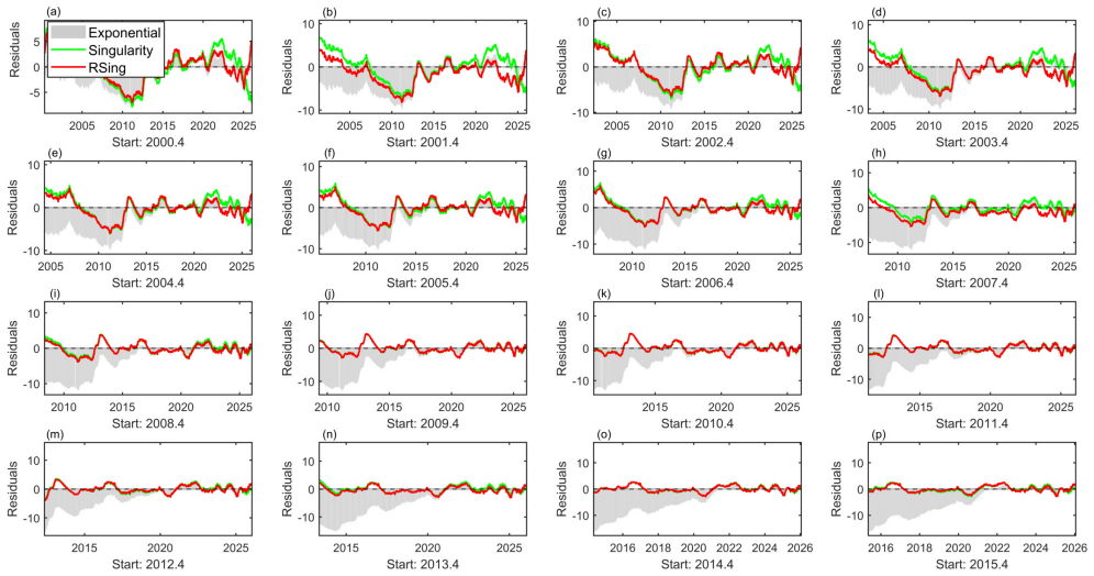
For detailed average values with uncertainty, see Table 3. 19/46 Figure 10.Comparison of the finite-time singularity and regularized singularity models for GNSS vertical displacement at station RITE. (a) Estimated critical time tc as a function of analysis start date for both models. The regularized model yields tc values systematically closer to the pres...
work page 2008
discussion (0)
Sign in with ORCID, Apple, or X to comment. Anyone can read and Pith papers without signing in.