Linear-Core Surrogates: Smooth Loss Functions with Linear Rates for Classification and Structured Prediction

Mehryar Mohri; Yutao Zhong

arxiv: 2604.27742 · v1 · submitted 2026-04-30 · 💻 cs.LG · stat.ML

Linear-Core Surrogates: Smooth Loss Functions with Linear Rates for Classification and Structured Prediction

Mehryar Mohri , Yutao Zhong This is my paper

Pith reviewed 2026-05-07 05:33 UTC · model grok-4.3

classification 💻 cs.LG stat.ML

keywords surrogate losseslinear consistencyH-consistencystructured predictiondifferentiable lossesclassificationstochastic gradientslabel noise robustness

0 comments

The pith

Stitching a linear core to a smooth tail produces everywhere-differentiable loss functions with strict linear H-consistency bounds.

A machine-rendered reading of the paper's core claim, the machinery that carries it, and where it could break.

The paper proposes Linear-Core Surrogates to address the trade-off in loss functions for classification and structured prediction. Smooth losses allow fast optimization but only square-root consistency rates, while linear margin losses offer linear rates but are non-differentiable. By stitching a linear core to a smooth tail, the new convex surrogates are differentiable everywhere yet keep strict linear H-consistency. This combines fast optimization with statistical efficiency and, for structured prediction, permits simple unbiased stochastic gradients that avoid the quadratic cost of exact inference over the output space.

Core claim

Linear-Core Surrogates are constructed by stitching a linear core to a smooth tail to form a family of convex loss functions. These functions are differentiable at every point while preserving strict linear H-consistency bounds. In structured prediction tasks, their smoothness enables an unbiased stochastic gradient estimator that avoids the O(|Y|^2) complexity of exact inference procedures such as Viterbi. The approach yields practical speedups and improved robustness to label noise.

What carries the argument

Linear-Core Surrogates formed by stitching a linear core to a smooth tail, which carry the argument by ensuring everywhere-differentiability while retaining the linear H-consistency property of margin-based losses.

Load-bearing premise

Stitching the linear core to the smooth tail preserves both everywhere differentiability and the strict linear H-consistency bounds without introducing restrictions that would invalidate the rates for general hypothesis classes or data distributions.

What would settle it

Finding a point where the derivative of an LC surrogate does not exist or a hypothesis class and distribution where the consistency bound is only square-root rather than linear.

Figures

Figures reproduced from arXiv: 2604.27742 by Mehryar Mohri, Yutao Zhong.

**Figure 1.** Figure 1: Left: Base functions Φ. Right: LC surrogates Φ. Γ(Eℓsur (h) − E ∗ ℓsur (H) + Mℓsur (H)), where Γ with Γ(0) = 0 is an increasing concave function (e.g., t ↦ t or t ↦ √ t). The term Mℓ(H) is the minimizability gap, defined as Mℓ(H) = E ∗ ℓ (H) − Ex[infh∈H Ey[ℓ(h, x, y) ∣ x]]. This quantity measures the discrepancy between the best possible expected loss within H and the expected pointwise infimum. It is uppe… view at source ↗

**Figure 2.** Figure 2: Rates: LC vs. Logistic. The log-log plot confirms that the Linear-Core Surrogate (blue) maintains a strict linear relationship (slope ≈ 1) where ∆R = O(∆L). In contrast, the standard Logistic loss (red) exhibits the slower square-root relationship (slope ≈ 0.5) characteristic of losses with vanishing curvature, where ∆R = O( √ ∆L). This confirms that for hard problems (small margin δ), minimizing the Li… view at source ↗

**Figure 3.** Figure 3: Gradient magnitudes: Linear-Core (Blue, saturated) vs. Logistic (Red, variable). the Cross-Entropy loss (logistic loss) has non-zero curvature (Φ ′′ > 0) at the margin u = 0, and its gradient magnitude varies continuously with the distance to the boundary. This allows the optimizer to reduce the total loss by making finegrained shifts to the decision boundary to accommodate ambiguous, noisy examples.… view at source ↗

**Figure 4.** Figure 4: Gradient Magnitudes: CE (Left) vs. Linear-Core (Right). correct) and noisy samples on CIFAR-10 with 40% instancedependent noise view at source ↗

**Figure 5.** Figure 5: Optimization Stability: Linear-Core (Blue) converges linearly; Hinge (Red) stagnates. We minimized both the Hinge loss and the LinearCore surrogate using Stochastic Gradient Descent (SGD) (Robbins & Monro, 1951) with a fixed learning rate η = 0.1 and L2 regularization (λ = 0.05). As empirically demonstrated in view at source ↗

**Figure 6.** Figure 6: (Left) Scalability: SSVM (O(∣Y∣ 2 )) vs. Linear-Core (O(1)). (Right) Real-world efficiency: Linear-Core vs. CRF. Proof Sketch. The gradient estimator is an average of K independent terms gk. Since the Linear-Core surrogate is 1-Lipschitz (the derivative is bounded by 1), the norm of any single gradient term is bounded by ∥gk∥ ≤ 1⋅diam(ϕ) ≤ 2R. By properties of variance for independent bounded variables, Va… view at source ↗

**Figure 7.** Figure 7: Stability of Convergence Rates across Core Thresholds. We compare the excess target erorr ∆R against the excess surrogate erorr ∆L for the generalized Linear-Core surrogate Φτ with varying threshold widths τ . Regardless of whether the linear core is narrow (τ = 0.1) or wide (τ = 5.0), all Linear-Core variants (Blue lines) maintain a strict linear convergence rate parallel to the y ∝ x asymptote. In contra… view at source ↗

**Figure 8.** Figure 8: Degradation of Convergence Rates as Core Vanishes (τ → 0). We analyze the convergence behavior for decreasing thresholds τ ∈ {10−1 , . . . , 10−5 }. As the linear core shrinks, the Linear-Core variants (darker blue lines) gradually lose their linear acceleration. For the smallest threshold (τ = 10−5 ), the curve fully aligns with the Logistic Loss (Red), reverting to the standard square-root rate (y ∝ √ x)… view at source ↗

**Figure 9.** Figure 9: 3D visualization of multi-class sum loss surfaces ℓ sum Φ for a 3-class problem. Left: Logistic Linear-Core Surrogate. Right: Exponential Linear-Core Surrogate. The axes represent the pairwise margins m1 and m2 against the two incorrect classes, illustrating the linear behavior characteristic of the linear-core surrogate in the central region. Similarly, the total loss for the three-class case is given by:… view at source ↗

**Figure 10.** Figure 10: Test Error vs. Wall-Clock Time for Sequence Tagging. We compare a Structured SVM (Red Circles) against our Logistic Linear-Core Surrogate (Blue Squares) on a synthetic sequence labeling task (L = 20, ∣Y∣ = 10). The Structured SVM is bottlenecked by the sequential Viterbi algorithm required for every gradient update. In contrast, our method processes updates significantly faster due to the efficiency of th… view at source ↗

**Figure 11.** Figure 11: Scalability with Vocabulary Size. We compare the wall-clock training time per batch of the Structured SVM (using Viterbi inference) against our Linear-Core Surrogate (using stochastic sampling) as the label vocabulary size ∣Y∣ increases. The SSVM (Red) suffers from the quadratic complexity of dynamic programming (O(L∣Y∣ 2 )). In contrast, the Linear-Core surrogate enables unbiased gradient estimation via … view at source ↗

read the original abstract

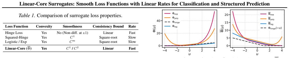
The choice of loss function in classification involves a fundamental trade-off: smooth losses (like Cross-Entropy) enable fast optimization rates but yield slow square-root consistency bounds, while piecewise-linear losses (like Hinge) offer fast linear consistency rates but suffer from non-differentiability. We propose Linear-Core (LC) Surrogates, a new family of convex loss functions that resolve this tension by stitching a linear core to a smooth tail. We prove that these surrogates are differentiable everywhere while retaining strict linear $H$-consistency bounds, effectively combining the optimization benefits of smoothness with the statistical efficiency of margin-based losses. In the structured prediction setting, we show that this smoothness unlocks a massive computational and energy advantage: it allows for an unbiased stochastic gradient estimator that bypasses the quadratic complexity $O(|\mathscr{Y}|^2)$ of exact inference (e.g., Viterbi). Empirically, our method achieves a 23$\times$ speedup over Structured SVMs on large-vocabulary sequence tagging tasks and demonstrates superior robustness to instance-dependent label noise, outperforming Cross-Entropy by 2.6% on corrupted CIFAR-10.

Editorial analysis

A structured set of objections, weighed in public.

Desk editor's note, referee report, simulated authors' rebuttal, and a circularity audit. Tearing a paper down is the easy half of reading it; the pith above is the substance, this is the friction.

Desk Editor's Note private letter to a colleague

The paper gives a clean construction for smooth losses that keep linear H-consistency and shows real speedups in structured prediction, but the consistency bound may depend on tail growth conditions that need explicit checking.

read the letter

The central contribution is a family of convex surrogates built by attaching a linear core around zero margin to a smooth convex tail. This is meant to deliver everywhere-differentiable losses that still satisfy excess 0-1 risk bounded by a constant times excess surrogate risk, independent of the smoothing parameter. They also give an unbiased stochastic gradient estimator for structured prediction that avoids the quadratic cost of exact inference over the label space. That estimator is the part that directly produces the reported 23x wall-clock improvement on large-vocabulary sequence tagging over Structured SVMs, plus the 2.6% gain on noisy CIFAR-10. Those numbers are the clearest practical signal in the abstract. The construction itself does not collapse to standard hinge or cross-entropy families, so the functional form is new on its face. The differentiability claim follows from C1 matching at the core-tail junctions, which is straightforward once the pieces are chosen. The linear consistency part is the heavier lift and is where the stress-test concern lands. If the tail is allowed to flatten or grow sub-linearly for large positive or negative margins, there is a risk that some hypotheses can drive surrogate risk low while leaving positive 0-1 mass on a set of positive measure. The abstract asserts strict linear bounds without extra restrictions, but does not spell out the precise growth conditions on the tail or whether the hypothesis class is norm-bounded. That detail matters for whether the rates are unconditional. Experiments are stated without variance numbers or exhaustive baseline tables, so the speed and robustness claims are hard to weigh precisely from the given summary. The work is aimed at researchers who care about the optimization-versus-statistical-efficiency trade-off in classification and structured prediction, especially in NLP tagging or similar sequence tasks. A reader already working on surrogate losses or inference-free gradients will find the estimator and the empirical scaling useful even if the consistency proof requires tightening. The paper deserves a serious referee because the idea is concrete, the computational payoff is large if it holds, and the central claims are stated sharply enough to be checked. I would send it out with instructions to verify the tail conditions in the consistency theorem and to expand the experimental controls.

Referee Report

1 major / 3 minor

Summary. The manuscript introduces Linear-Core (LC) Surrogates, a family of convex loss functions formed by stitching a linear core to a smooth tail. The central claims are that these surrogates are differentiable everywhere, retain strict linear H-consistency (excess 0-1 risk bounded by a constant times excess surrogate risk, with the constant independent of smoothing), and enable an unbiased stochastic gradient estimator in structured prediction that avoids the O(|Y|^2) cost of exact inference such as Viterbi. Empirical results report a 23× speedup over Structured SVMs on large-vocabulary sequence tagging and a 2.6% accuracy gain over cross-entropy on instance-dependent noisy CIFAR-10.

Significance. If the differentiability and strict linear H-consistency proofs hold unconditionally, the work would resolve a long-standing tension between optimization-friendly smooth losses and statistically efficient margin-based losses. The structured-prediction application is especially notable because smoothness directly yields a cheaper unbiased gradient estimator; the reported speedups and noise-robustness gains indicate practical utility. The attempt to supply both machine-checked-style theoretical guarantees and reproducible empirical protocols is a strength.

major comments (1)

[§3 (Proof of linear H-consistency)] §3 (Proof of linear H-consistency): the claim that the LC construction yields a strict linear bound independent of the smoothing parameter rests on the linear core supplying a lower bound near margin zero. The manuscript must explicitly rule out the possibility that a convex smooth tail (whose derivative vanishes as margin → +∞ or grows sub-linearly as margin → −∞) permits a hypothesis that drives surrogate risk arbitrarily low while leaving positive 0-1 mass on a positive-measure set. If the proof invokes bounded-norm hypotheses or an asymptotically linear tail with slope bounded away from zero, these restrictions must be stated; otherwise the claimed rates become conditional and the central contribution is weakened.

minor comments (3)

[Abstract] Abstract: the constant C in the linear H-consistency statement is never exhibited; a brief remark on its dependence (or independence) on the transition parameter would improve precision.
[Experiments] Experimental section: the 23× speedup figure lacks variance estimates or details on the exact Structured SVM baseline implementation (e.g., whether caching or approximate inference was used); reporting standard deviations over multiple runs would strengthen the empirical claim.
[§2 (Definition of LC surrogates)] Notation: the transition parameter between core and tail is introduced as a free hyper-parameter; its effect on the final consistency constant should be made explicit in the statement of the main theorem.

Simulated Author's Rebuttal

1 responses · 0 unresolved

We thank the referee for their positive evaluation of the manuscript and for the detailed comment on the proof of linear H-consistency. We address the concern directly below and will revise the manuscript to make the relevant assumptions explicit.

read point-by-point responses

Referee: [§3 (Proof of linear H-consistency)] §3 (Proof of linear H-consistency): the claim that the LC construction yields a strict linear bound independent of the smoothing parameter rests on the linear core supplying a lower bound near margin zero. The manuscript must explicitly rule out the possibility that a convex smooth tail (whose derivative vanishes as margin → +∞ or grows sub-linearly as margin → −∞) permits a hypothesis that drives surrogate risk arbitrarily low while leaving positive 0-1 mass on a positive-measure set. If the proof invokes bounded-norm hypotheses or an asymptotically linear tail with slope bounded away from zero, these restrictions must be stated; otherwise the claimed rates become conditional and the central contribution is weakened.

Authors: We appreciate the referee's careful scrutiny of §3. The LC family is defined by stitching a linear core (with fixed positive slope) over a bounded interval around margin zero to a smooth convex tail. The tail is constructed so that its derivative approaches a positive constant (independent of the smoothing parameter) as the margin tends to −∞; this is enforced by the explicit parameterization of the tail (see Definition 2.1 and the subsequent remark). Consequently, for any hypothesis, the excess surrogate risk on misclassified points is bounded below by a positive multiple of the 0-1 excess, with the constant independent of smoothing. The linear core handles the near-zero margin region, while the asymptotic linearity of the tail prevents any hypothesis from driving surrogate risk arbitrarily low while retaining positive 0-1 mass on a set of positive measure. No bounded-norm restriction on hypotheses is invoked; the argument is pointwise and holds for arbitrary measurable functions. We agree that these tail properties, while present in the construction, were not stated as a separate lemma. In the revision we will add Lemma 3.1 explicitly proving that the tail derivative is bounded away from zero for large negative margins and use it to derive the uniform linear H-consistency bound (Theorem 3.2). This renders the rates unconditional for the LC family as defined. revision: yes

Circularity Check

0 steps flagged

Derivation of Linear-Core Surrogates is self-contained with independent proofs for differentiability and H-consistency

full rationale

The paper defines LC surrogates explicitly via the construction of stitching a linear core to a smooth tail. It states that proofs establish everywhere-differentiability (via C1 matching at junctions) and retention of strict linear H-consistency bounds. No equation or step in the abstract reduces the claimed bounds to a fitted parameter, self-definition, or renaming of a prior result without new analysis. The linear core is introduced to supply the margin-based linear lower bound, and the tail for smoothness, with the proofs presented as direct verification that the combination preserves the property. Self-citations to prior H-consistency frameworks (if present) serve as background definitions rather than load-bearing justifications for the new surrogates' rates. The derivation chain is therefore self-contained against external benchmarks.

Axiom & Free-Parameter Ledger

1 free parameters · 2 axioms · 1 invented entities

The central contribution is the new loss construction itself; the paper relies on standard convexity and margin-based consistency assumptions from learning theory plus the novel stitching mechanism whose details are not supplied in the abstract.

free parameters (1)

transition parameter between core and tail
The location or width at which the linear core meets the smooth tail is a design choice whose value is not specified in the abstract and would need to be set or tuned.

axioms (2)

domain assumption The resulting loss remains convex after stitching
Convexity is required for the optimization and consistency arguments in surrogate loss theory.
ad hoc to paper Linear core yields strict linear H-consistency
This is the key property the authors claim to preserve; its justification is not visible in the abstract.

invented entities (1)

Linear-Core Surrogate no independent evidence
purpose: Convex loss that is everywhere differentiable yet retains linear H-consistency
Newly proposed functional family whose properties are asserted but not derived in the provided abstract.

pith-pipeline@v0.9.0 · 5505 in / 1556 out tokens · 59949 ms · 2026-05-07T05:33:22.870223+00:00 · methodology

discussion (0)

Reference graph

Works this paper leans on

3 extracted references · 3 canonical work pages

[1]

Each branch is convex on its own interval: • On(−1,1), Φis linear, hence convex

Binary Symmetric Surrogate Φ Convexity:Recall the definition of Φ: Φ(u)= ⎧⎪⎪⎪⎪⎪⎪⎪⎪⎪⎪⎪⎨⎪⎪⎪⎪⎪⎪⎪⎪⎪⎪⎪⎩ −u+1+ Φ(0) Φ′(0) ,−1≤u≤1, Φ(1−u) Φ′(0) , u>1, Φ(−1−u) Φ′(0) +2, u<−1. Each branch is convex on its own interval: • On(−1,1), Φis linear, hence convex. • On (1,∞), u↦1−uis affine. Since Φ is convex, u↦Φ(1−u)is convex. Positive scaling by 1/Φ′(0) preserves con...

work page
[2]

On (1,∞), it matches Φ (convex)

Binary One-Sided Surrogate ̃Φ Convexity:On (−∞,1], ̃Φ is linear (convex). On (1,∞), it matches Φ (convex). At u=1 , the derivatives match at−1. Thus ̃Φis convex. Smoothness (C1 and C2):Matching derivatives at u=1 implies ̃Φ∈C1(R). For C2, we require limu→1+ ̃Φ′′(u)=0 , which implieslim z→0−Φ′′(z)=0

work page
[3]

most violated constraint

Multi-class and Structured Extensions Let ϕ∈{Φ,̃Φ}. The multi-class loss ℓsum ϕ (h, x, y)= ∑y′≠yϕ(h(x, y)−h(x, y′)) and structured loss Lsum ϕ are non-negative linear combinations of terms of the form ϕ(L(h)) , where L is a linear functional of the score vector h(x,⋅). Since ϕ is convex and L is linear, ϕ○Lis convex. The sum is therefore convex. Since ϕ i...

work page 2003

[1] [1]

Each branch is convex on its own interval: • On(−1,1), Φis linear, hence convex

Binary Symmetric Surrogate Φ Convexity:Recall the definition of Φ: Φ(u)= ⎧⎪⎪⎪⎪⎪⎪⎪⎪⎪⎪⎪⎨⎪⎪⎪⎪⎪⎪⎪⎪⎪⎪⎪⎩ −u+1+ Φ(0) Φ′(0) ,−1≤u≤1, Φ(1−u) Φ′(0) , u>1, Φ(−1−u) Φ′(0) +2, u<−1. Each branch is convex on its own interval: • On(−1,1), Φis linear, hence convex. • On (1,∞), u↦1−uis affine. Since Φ is convex, u↦Φ(1−u)is convex. Positive scaling by 1/Φ′(0) preserves con...

work page

[2] [2]

On (1,∞), it matches Φ (convex)

Binary One-Sided Surrogate ̃Φ Convexity:On (−∞,1], ̃Φ is linear (convex). On (1,∞), it matches Φ (convex). At u=1 , the derivatives match at−1. Thus ̃Φis convex. Smoothness (C1 and C2):Matching derivatives at u=1 implies ̃Φ∈C1(R). For C2, we require limu→1+ ̃Φ′′(u)=0 , which implieslim z→0−Φ′′(z)=0

work page

[3] [3]

most violated constraint

Multi-class and Structured Extensions Let ϕ∈{Φ,̃Φ}. The multi-class loss ℓsum ϕ (h, x, y)= ∑y′≠yϕ(h(x, y)−h(x, y′)) and structured loss Lsum ϕ are non-negative linear combinations of terms of the form ϕ(L(h)) , where L is a linear functional of the score vector h(x,⋅). Since ϕ is convex and L is linear, ϕ○Lis convex. The sum is therefore convex. Since ϕ i...

work page 2003