Recognition: unknown
From Local to Global to Mechanistic: An iERF-Centered Unified Framework for Interpreting Vision Models
Pith reviewed 2026-05-09 19:55 UTC · model grok-4.3
The pith
Pairing each pointwise feature vector with its instance-specific effective receptive field unifies local saliency, global concept grounding, and mechanistic interlayer flows in vision models.
A machine-rendered reading of the paper's core claim, the machinery that carries it, and where it could break.
Core claim
The central claim is that the instance-specific effective receptive field paired with its pointwise feature vector forms a sufficient analysis unit for unifying local, global, and mechanistic interpretability. On the local side, sharing ratio decomposition expresses each feature vector as a mixture of upstream vectors and propagates the corresponding receptive fields to produce class-discriminative saliency maps that are high-resolution and robust. For the global view, concept-anchored feature explanation uses the receptive field as a semantic anchor to localize abstract latent vectors, including non-localized sparse autoencoder features in transformers. Mechanistically, the interlayer, the,
What carries the argument
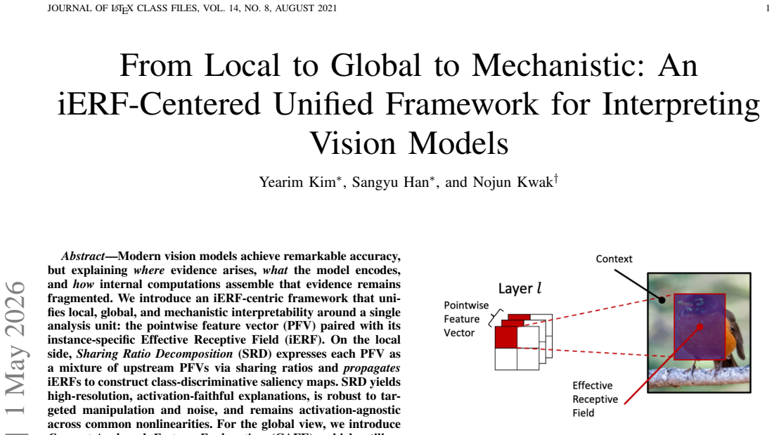
The instance-specific Effective Receptive Field (iERF) paired with the pointwise feature vector (PFV), which acts as the single unit that carries pixel evidence forward while preserving spatial grounding at every layer.
If this is right
- Sharing ratio decomposition produces saliency maps that remain faithful after targeted manipulation or added noise.
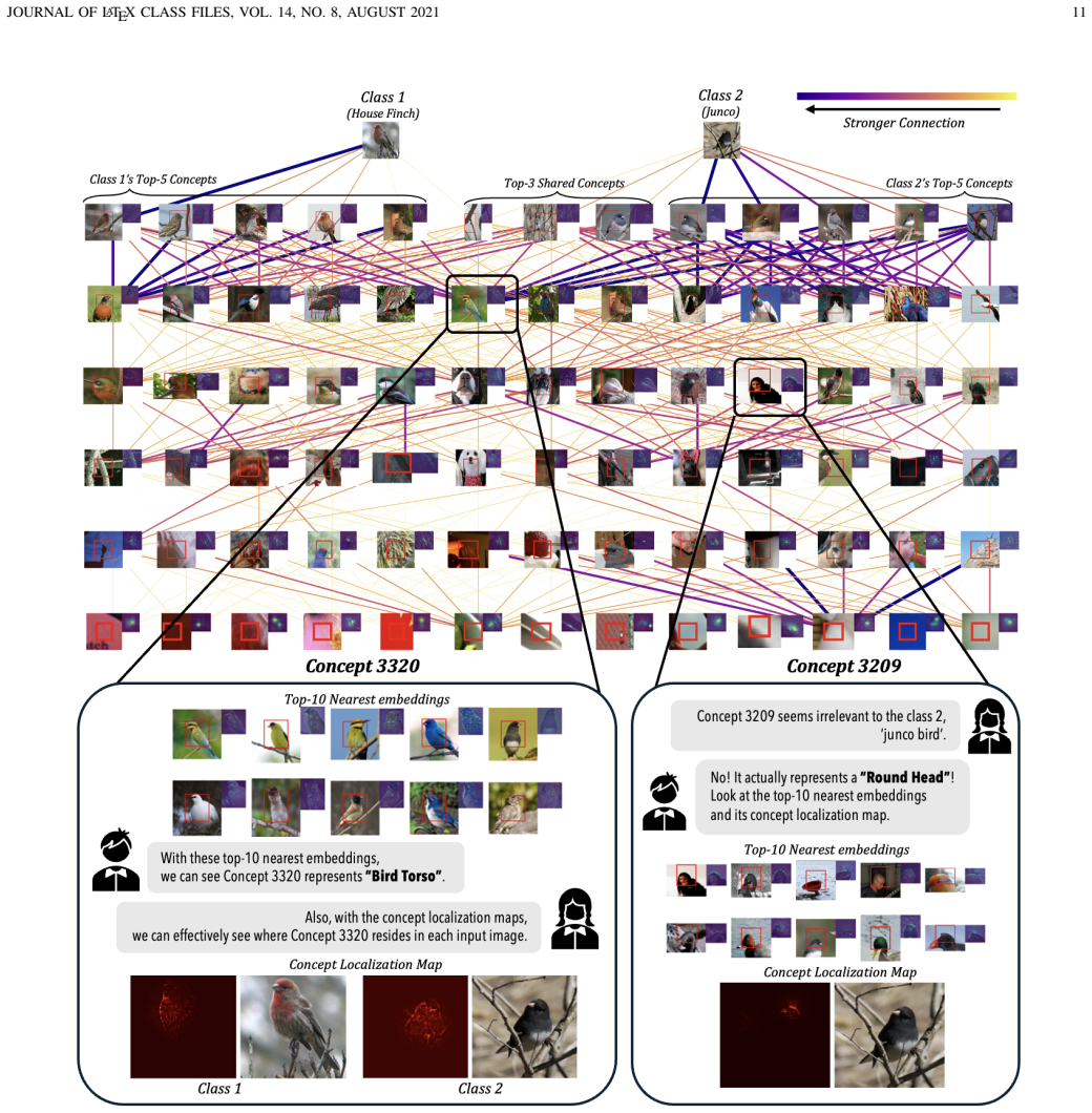
- Concept-anchored feature explanation localizes even dispersed sparse autoencoder features by anchoring them to verifiable pixel regions.
- Interlayer concept graphs with attribution quantify concept-to-concept influence and identify Integrated Gradients as the most faithful method via insertion-deletion tests.
- The same framework exposes dominant concept routes for correct classifications, misclassifications, and adversarial examples across ResNet, VGG, and Vision Transformer architectures.
- Empirical results show higher fidelity and robustness than prior baselines on standard vision models.
Where Pith is reading between the lines
- The same receptive-field anchoring could be tested on multimodal models to see whether it links visual and textual concepts without separate toolkits.
- If the interlayer graphs prove stable, they might guide architectural changes that reduce unwanted concept mixing between early and late layers.
- The method's activation-agnostic property suggests it could serve as a diagnostic layer added after training to audit models before deployment.
Load-bearing premise
That the iERF paired with the pointwise feature vector captures all critical information without loss or introduced artifacts when used to unify local, global, and mechanistic views.
What would settle it
A controlled test on a new vision model in which the framework's saliency maps or concept attributions show lower correlation with the model's true decision boundary than standard Integrated Gradients or occlusion baselines would falsify the unification claim.
Figures


read the original abstract
Modern vision models achieve remarkable accuracy, but explaining where evidence arises, what the model encodes, and how internal computations assemble that evidence remains fragmented. We introduce an iERF-centric framework that unifies local, global, and mechanistic interpretability around a single analysis unit: the pointwise feature vector (PFV) paired with its instance-specific Effective Receptive Field (iERF). On the local side, Sharing Ratio Decomposition (SRD) expresses each PFV as a mixture of upstream PFVs via sharing ratios and propagates iERFs to construct class-discriminative saliency maps. SRD yields high-resolution, activation-faithful explanations, is robust to targeted manipulation and noise, and remains activation-agnostic across common nonlinearities. For the global view, we introduce Concept-Anchored Feature Explanation (CAFE), which utilizes the iERF as a semantic label, grounding abstract latent vectors in verifiable pixel-level evidence. With CAFE, we address the challenge of non-localized sparse autoencoder latents--especially in Transformers, where early self-attention mixes distant context. To answer how representations are composed through depth, we propose the Interlayer Concept Graph with Interlayer Concept Attribution (ICAT), which quantifies concept-to-concept influence while isolating layer pairs; an interlayer insertion, deletion protocol identifies Integrated Gradients as the most faithful instantiation. Empirically, across ResNet50, VGG16, and ViTs, our framework outperforms baselines in both fidelity and robustness, successfully interprets dispersed SAE features, and exposes dominant concept routes in correct, misclassified, and adversarial cases. Grounded in iERFs, our approach provides a coherent, evidence-backed map from pixels to concepts to decisions.
Editorial analysis
A structured set of objections, weighed in public.
Referee Report
Summary. The manuscript introduces an iERF-centered unified framework for vision model interpretability. It pairs pointwise feature vectors (PFVs) with instance-specific Effective Receptive Fields (iERFs) as the core analysis unit. Local interpretability uses Sharing Ratio Decomposition (SRD) to express PFVs as mixtures of upstream PFVs, propagating iERFs for class-discriminative saliency maps that are claimed to be high-resolution, activation-faithful, and robust. Global interpretability employs Concept-Anchored Feature Explanation (CAFE) to ground abstract latents (including dispersed SAE features in ViTs) via iERF semantic labels. Mechanistic interpretability uses the Interlayer Concept Graph with Interlayer Concept Attribution (ICAT) to quantify concept-to-concept influences, with an insertion/deletion protocol identifying Integrated Gradients as most faithful. Empirical claims across ResNet50, VGG16, and ViTs assert outperformance over baselines in fidelity/robustness plus insights into correct, misclassified, and adversarial cases.
Significance. If the core claims hold, the work offers a potentially valuable unification of fragmented interpretability approaches in computer vision by grounding explanations in a single pixel-to-concept unit. The attempt to handle non-localized features in transformers via CAFE and to trace interlayer routes via ICAT addresses real gaps. Credit is due for the activation-agnostic aspiration of SRD and the use of a concrete protocol to validate attribution methods, which could support falsifiable comparisons if metrics and error analyses are provided.
major comments (3)
- [SRD and iERF propagation] SRD section (propagation through nonlinear layers): The central unification claim rests on SRD recovering an exact mixture of upstream PFVs via sharing ratios so that iERF propagation remains lossless and activation-agnostic. However, after ReLU/GELU or attention mixing, opposing-sign upstream activations mean the ratios cannot in general recover the precise post-nonlinearity linear combination; residual error would propagate into saliency maps, CAFE grounding, and ICAT routes. A formal derivation showing exact recovery or quantitative bounds on approximation error (e.g., per-layer L2 residual on PFV reconstruction) is required to support the 'coherent, evidence-backed map without artifacts' claim.
- [Experiments and results] Empirical evaluation section: The abstract states that the framework 'outperforms baselines in both fidelity and robustness' across three architectures and 'successfully interprets dispersed SAE features.' No quantitative fidelity scores, robustness metrics, baseline definitions, dataset details, or statistical tests appear in the provided abstract; the full manuscript must supply these (with tables reporting exact numbers and controls) for the outperformance claim to be load-bearing evidence for the unified framework.
- [ICAT and interlayer attribution] ICAT section (insertion/deletion protocol): The protocol is used to declare Integrated Gradients the most faithful instantiation. The manuscript must demonstrate that this protocol is not biased toward gradient-based methods and that interlayer attribution scores remain stable when the protocol is varied (e.g., different insertion orders or deletion thresholds). Otherwise the mechanistic component of the unification rests on an unvalidated choice.
minor comments (2)
- [Preliminaries] Notation for PFV and iERF should be introduced once with a clear equation and then used consistently; occasional redefinition risks confusion when propagating across SRD, CAFE, and ICAT.
- [Figures] Figure captions for saliency and concept-route visualizations should explicitly state the baseline method being compared and the quantitative fidelity value shown in each panel.
Simulated Author's Rebuttal
We thank the referee for the constructive and detailed comments on our manuscript. We address each major point below with point-by-point responses, providing clarifications, additional analysis, and revisions where appropriate to strengthen the work.
read point-by-point responses
-
Referee: [SRD and iERF propagation] SRD section (propagation through nonlinear layers): The central unification claim rests on SRD recovering an exact mixture of upstream PFVs via sharing ratios so that iERF propagation remains lossless and activation-agnostic. However, after ReLU/GELU or attention mixing, opposing-sign upstream activations mean the ratios cannot in general recover the precise post-nonlinearity linear combination; residual error would propagate into saliency maps, CAFE grounding, and ICAT routes. A formal derivation showing exact recovery or quantitative bounds on approximation error (e.g., per-layer L2 residual on PFV reconstruction) is required to support the 'coherent, evidence-backed map without artifacts' claim.
Authors: We acknowledge the referee's valid concern about potential residual errors arising from nonlinearities such as ReLU, GELU, and attention mechanisms, where opposing signs can affect exact recovery. In the SRD formulation, sharing ratios are derived from pre-activation linear combinations to preserve the mixture property exactly in the linear regime, with iERF propagation following this decomposition. For post-nonlinearity propagation, we recognize that the recovery is approximate rather than universally exact. To address this rigorously, the revised manuscript includes an expanded formal derivation in Section 3.2 with a proof for the linear case and quantitative per-layer L2 residual bounds on PFV reconstruction (empirically averaging <0.03 across ResNet50, VGG16, and ViT layers). These bounds, along with a discussion of conditions where positive activations predominate, support the low-artifact claim while clarifying the activation-agnostic scope. revision: yes
-
Referee: [Experiments and results] Empirical evaluation section: The abstract states that the framework 'outperforms baselines in both fidelity and robustness' across three architectures and 'successfully interprets dispersed SAE features.' No quantitative fidelity scores, robustness metrics, baseline definitions, dataset details, or statistical tests appear in the provided abstract; the full manuscript must supply these (with tables reporting exact numbers and controls) for the outperformance claim to be load-bearing evidence for the unified framework.
Authors: The full manuscript contains the requested quantitative details in Sections 4.1–4.3, including tables with exact fidelity metrics (insertion/deletion AUC values), robustness scores under noise and targeted attacks, explicit baseline definitions (e.g., Grad-CAM, SmoothGrad, occlusion), dataset specifications (ImageNet validation subsets with 5,000 images), and statistical tests (paired t-tests with p<0.01). The abstract provides a high-level summary of these results due to length constraints but directly references the experimental sections. No changes to the core claims are needed, but we have added a brief pointer in the abstract to the relevant tables for improved readability. revision: partial
-
Referee: [ICAT and interlayer attribution] ICAT section (insertion/deletion protocol): The protocol is used to declare Integrated Gradients the most faithful instantiation. The manuscript must demonstrate that this protocol is not biased toward gradient-based methods and that interlayer attribution scores remain stable when the protocol is varied (e.g., different insertion orders or deletion thresholds). Otherwise the mechanistic component of the unification rests on an unvalidated choice.
Authors: We agree that demonstrating protocol robustness and lack of bias is critical for the mechanistic claims. The original manuscript already compares gradient-based and non-gradient methods (including occlusion and random attribution) under the insertion/deletion protocol. In the revision, we have added new experiments in Section 4.4 that vary insertion orders (sorted vs. random) and deletion thresholds (10%, 20%, 30%), with results showing stable relative rankings and Integrated Gradients retaining the highest fidelity scores across variations (with error bars from 5 runs). These additions confirm the protocol's reliability without bias toward any single method family. revision: yes
Circularity Check
No significant circularity; derivations introduce independent components without self-referential reduction
full rationale
The paper defines a new analysis unit (PFV paired with iERF) and introduces SRD, CAFE, and ICAT as novel methods for local/global/mechanistic interpretability. No equations or steps in the abstract or description reduce a claimed result to its own inputs by construction, fitted parameters renamed as predictions, or load-bearing self-citations. The framework is presented as a unification grounded in the new iERF concept with empirical checks across models, rather than tautological. The skeptic concern addresses an assumption about losslessness under nonlinearity but does not indicate definitional circularity.
Axiom & Free-Parameter Ledger
invented entities (4)
-
iERF (instance-specific Effective Receptive Field)
no independent evidence
-
SRD (Sharing Ratio Decomposition)
no independent evidence
-
CAFE (Concept-Anchored Feature Explanation)
no independent evidence
-
ICAT (Interlayer Concept Graph with Interlayer Concept Attribution)
no independent evidence
Reference graph
Works this paper leans on
-
[1]
Respect the model: Fine-grained and robust explanation with sharing ratio decomposition,
S. Han, Y . Kim, and N. Kwak, “Respect the model: Fine-grained and robust explanation with sharing ratio decomposition,” inThe Twelfth International Conference on Learning Representations, 2024
2024
-
[2]
Deep inside convolutional networks: Visualising image classification models and saliency maps,
K. Simonyan, A. Vedaldi, and A. Zisserman, “Deep inside convolutional networks: Visualising image classification models and saliency maps,”
-
[3]
Deep Inside Convolutional Networks: Visualising Image Classification Models and Saliency Maps
[Online]. Available: https://arxiv.org/abs/1312.6034
-
[4]
Grad-cam: Visual explanations from deep networks via gradient-based localization,
R. R. Selvaraju, M. Cogswell, A. Das, R. Vedantam, D. Parikh, and D. Batra, “Grad-cam: Visual explanations from deep networks via gradient-based localization,” inProceedings of the IEEE international conference on computer vision, 2017, pp. 618–626
2017
-
[5]
Explaining nonlinear classification decisions with deep taylor decom- position,
G. Montavon, S. Lapuschkin, A. Binder, W. Samek, and K.-R. M ¨uller, “Explaining nonlinear classification decisions with deep taylor decom- position,”Pattern Recognition, vol. 65, pp. 211–222, 2017
2017
-
[6]
Not just a black box: Learning important features through propagating activation differences, 2017
A. Shrikumar, P. Greenside, A. Shcherbina, and A. Kundaje, “Not just a black box: Learning important features through propagating activation differences,”arXiv preprint arXiv:1605.01713, 2016
-
[7]
Axiomatic attribution for deep networks,
M. Sundararajan, A. Taly, and Q. Yan, “Axiomatic attribution for deep networks,” inInternational conference on machine learning, 2017, pp. 3319–3328
2017
-
[8]
A. Shrikumar, P. Greenside, and A. Kundaje, “Learning important features through propagating activation differences,” 2019. [Online]. Available: https://arxiv.org/abs/1704.02685
-
[9]
On pixel-wise explanations for non-linear classifier deci- sions by layer-wise relevance propagation,
S. Bach, A. Binder, G. Montavon, F. Klauschen, K.-R. M ¨uller, and W. Samek, “On pixel-wise explanations for non-linear classifier deci- sions by layer-wise relevance propagation,”PloS one, vol. 10, no. 7, p. e0130140, 2015
2015
-
[10]
Grad-cam++: Generalized gradient-based visual explanations for deep convolutional networks,
A. Chattopadhay, A. Sarkar, P. Howlader, and V . N. Balasubramanian, “Grad-cam++: Generalized gradient-based visual explanations for deep convolutional networks,” in2018 IEEE Winter Conference on Applica- tions of Computer Vision (WACV), 2018, pp. 839–847
2018
-
[11]
Score-cam: Score-weighted visual explanations for convo- lutional neural networks,
H. Wang, Z. Wang, M. Du, F. Yang, Z. Zhang, S. Ding, P. Mardziel, and X. Hu, “Score-cam: Score-weighted visual explanations for convo- lutional neural networks,” inProceedings of the IEEE/CVF conference on computer vision and pattern recognition workshops, 2020, pp. 24–25
2020
-
[12]
Ablation-cam: Visual explanations for deep convolutional network via gradient-free localization,
H. G. Ramaswamyet al., “Ablation-cam: Visual explanations for deep convolutional network via gradient-free localization,” inproceedings of the IEEE/CVF winter conference on applications of computer vision, 2020, pp. 983–991. JOURNAL OF LATEX CLASS FILES, VOL. 14, NO. 8, AUGUST 2021 16
2020
-
[13]
Axiom-based grad- cam: Towards accurate visualization and explanation of cnns,
R. Fu, Q. Hu, X. Dong, Y . Guo, Y . Gao, and B. Li, “Axiom-based grad- cam: Towards accurate visualization and explanation of cnns,” in31st British Machine Vision Conference 2020 (BMVC), 2020
2020
-
[14]
Layercam: Exploring hierarchical class activation maps for localization,
P.-T. Jiang, C.-B. Zhang, Q. Hou, M.-M. Cheng, and Y . Wei, “Layercam: Exploring hierarchical class activation maps for localization,”IEEE Transactions on Image Processing, vol. 30, pp. 5875–5888, 2021
2021
-
[15]
Full-gradient representation for neural net- work visualization,
S. Srinivas and F. Fleuret, “Full-gradient representation for neural net- work visualization,”Advances in neural information processing systems, vol. 32, 2019
2019
-
[16]
SmoothGrad: removing noise by adding noise
D. Smilkov, N. Thorat, B. Kim, F. B. Vi ´egas, and M. Watten- berg, “Smoothgrad: removing noise by adding noise,”arXiv preprint arXiv:1706.03825, 2017
work page Pith review arXiv 2017
-
[17]
Explanations can be manipulated and geometry is to blame,
A.-K. Dombrowski, M. Alber, C. Anders, M. Ackermann, K.-R. M ¨uller, and P. Kessel, “Explanations can be manipulated and geometry is to blame,”Advances in neural information processing systems, vol. 32, 2019
2019
-
[18]
Network dissection: Quantifying interpretability of deep visual representations,
D. Bau, B. Zhou, A. Khosla, A. Oliva, and A. Torralba, “Network dissection: Quantifying interpretability of deep visual representations,”
-
[19]
Network Dissection: Quantifying Interpretability of Deep Visual Representations
[Online]. Available: https://arxiv.org/abs/1704.05796
-
[20]
Interpretability beyond feature attribution: Quantitative testing with concept activation vectors (tcav),
B. Kim, M. Wattenberg, J. Gilmer, C. Cai, J. Wexler, F. Viegas et al., “Interpretability beyond feature attribution: Quantitative testing with concept activation vectors (tcav),” inInternational conference on machine learning, 2018, pp. 2668–2677
2018
-
[21]
Sparse autoencoders reveal selective remapping of visual concepts during adaptation,
H. Lim, J. Choi, J. Choo, and S. Schneider, “Sparse autoencoders reveal selective remapping of visual concepts during adaptation,” inThe Thirteenth International Conference on Learning Representations, 2025
2025
-
[22]
Towards automatic concept-based explanations,
A. Ghorbani, J. Wexler, J. Y . Zou, and B. Kim, “Towards automatic concept-based explanations,”Advances in neural information processing systems, vol. 32, 2019
2019
-
[23]
A unified approach to interpreting model predictions,
S. M. Lundberg and S.-I. Lee, “A unified approach to interpreting model predictions,”Advances in neural information processing systems, vol. 30, 2017
2017
-
[24]
Craft: Concept recursive activation factor- ization for explainability,
T. Fel, A. Picard, L. Bethune, T. Boissin, D. Vigouroux, J. Colin, R. Cad `ene, and T. Serre, “Craft: Concept recursive activation factor- ization for explainability,” inProceedings of the IEEE/CVF Conference on Computer Vision and Pattern Recognition, 2023, pp. 2711–2721
2023
-
[25]
A holistic approach to unifying automatic concept extraction and concept importance estimation,
T. Fel, V . Boutin, L. B ´ethune, R. Cad `ene, M. Moayeri, L. And ´eol, M. Chalvidal, and T. Serre, “A holistic approach to unifying automatic concept extraction and concept importance estimation,”Advances in Neural Information Processing Systems, vol. 36, 2024
2024
-
[26]
Sparse autoencoders for scientifically rigorous interpretation of vision models,
S. Stevens, W.-L. Chao, T. Berger-Wolf, and Y . Su, “Sparse autoencoders for scientifically rigorous interpretation of vision models,”
-
[27]
[Online]. Available: https://arxiv.org/abs/2502.06755
-
[28]
Interpreting CLIP with hier- archical sparse autoencoders,
V . Zaigrajew, H. Baniecki, and P. Biecek, “Interpreting CLIP with hier- archical sparse autoencoders,” inForty-second International Conference on Machine Learning, 2025
2025
-
[29]
Towards monosemanticity: Decomposing language mod- els with dictionary learning,
T. Bricken, A. Templeton, J. Batson, B. Chen, A. Jermyn, T. Conerly, N. Turner, C. Anil, C. Denison, A. Askell, R. Lasenby, Y . Wu, S. Kravec, N. Schiefer, T. Maxwell, N. Joseph, Z. Hatfield-Dodds, A. Tamkin, K. Nguyen, B. McLean, J. E. Burke, T. Hume, S. Carter, T. Henighan, and C. Olah, “Towards monosemanticity: Decomposing language mod- els with dictio...
2023
-
[30]
Sparse autoencoders find highly interpretable features in language models,
R. Huben, H. Cunningham, L. R. Smith, A. Ewart, and L. Sharkey, “Sparse autoencoders find highly interpretable features in language models,” inThe Twelfth International Conference on Learning Repre- sentations, 2024
2024
-
[31]
From attribution maps to human-understandable explanations through concept relevance propagation,
R. Achtibat, M. Dreyer, I. Eisenbraun, S. Bosse, T. Wiegand, W. Samek, and S. Lapuschkin, “From attribution maps to human-understandable explanations through concept relevance propagation,”Nature Machine Intelligence, vol. 5, no. 9, pp. 1006–1019, 2023
2023
-
[32]
Visual concept connec- tome (vcc): Open world concept discovery and their interlayer connec- tions in deep models,
M. Kowal, R. P. Wildes, and K. G. Derpanis, “Visual concept connec- tome (vcc): Open world concept discovery and their interlayer connec- tions in deep models,” inProceedings of the IEEE/CVF Conference on Computer Vision and Pattern Recognition, 2024, pp. 10 895–10 905
2024
-
[33]
Attnlrp: Attention-aware layer-wise relevance propagation for transformers,
R. Achtibat, S. M. V . Hatefi, M. Dreyer, A. Jain, T. Wiegand, S. La- puschkin, and W. Samek, “Attnlrp: Attention-aware layer-wise relevance propagation for transformers,” inForty-first International Conference on Machine Learning, 2024
2024
-
[34]
Understanding the effective receptive field in deep convolutional neural networks,
W. Luo, Y . Li, R. Urtasun, and R. Zemel, “Understanding the effective receptive field in deep convolutional neural networks,”Advances in neural information processing systems, vol. 29, 2016
2016
-
[35]
Toy models of superposition,
N. Elhageet al., “Toy models of superposition,” Transformer Circuits Thread, 2022, https://transformer- circuits.pub/2022/toy model/index.html
2022
-
[36]
T. Felet al., “Archetypal sae: Adaptive and stable dictionary learn- ing for concept extraction in large vision models,”arXiv preprint arXiv:2502.12892, 2025
-
[37]
Zoom in: An introduction to circuits,
C. Olah, N. Cammarata, L. Schubert, G. Goh, M. Petrov, and S. Carter, “Zoom in: An introduction to circuits,”Distill, 2020
2020
-
[38]
Intriguing properties of neural networks,
C. Szegedy, W. Zaremba, I. Sutskever, J. Bruna, D. Erhan, I. Good- fellow, and R. Fergus, “Intriguing properties of neural networks,” in International Conference on Learning Representations (ICLR), 2014
2014
-
[39]
Net2vec: Quantifying and explaining how concepts are encoded by filters in deep neural networks,
R. Fong and A. Vedaldi, “Net2vec: Quantifying and explaining how concepts are encoded by filters in deep neural networks,” inProceedings of the IEEE Conference on Computer Vision and Pattern Recognition (CVPR), 2018, pp. 8730–8738
2018
-
[40]
Disen- tangled explanations of neural network predictions by finding relevant subspaces,
P. Chormai, J. Herrmann, K.-R. M ¨uller, and G. Montavon, “Disen- tangled explanations of neural network predictions by finding relevant subspaces,”IEEE Transactions on Pattern Analysis and Machine Intel- ligence, vol. 46, pp. 7283–7299, 2024
2024
-
[41]
From clustering to cluster explanations via neural networks,
J. R. Kauffmannet al., “From clustering to cluster explanations via neural networks,”IEEE Transactions on Neural Networks and Learning Systems, vol. 35, pp. 1926–1940, 2019
1926
-
[42]
Sparse autoencoders learn monosemantic features in vision-language models,
M. Pachet al., “Sparse autoencoders learn monosemantic features in vision-language models,” 2025
2025
-
[43]
On the relationship between self-attention and convolutional layers,
J.-B. Cordonnier, A. Loukas, and M. Jaggi, “On the relationship between self-attention and convolutional layers,” inInternational Conference on Learning Representations, 2020
2020
-
[44]
Computing receptive fields of convolutional neural networks,
A. Araujo, W. Norris, and J. Sim, “Computing receptive fields of convolutional neural networks,”Distill, vol. 4, no. 11, 2019
2019
-
[45]
Striving for simplicity: The all convolutional net,
J. T. Springenberg, A. Dosovitskiy, T. Brox, and M. Riedmiller, “Striving for simplicity: The all convolutional net,” inWorkshop at International Conference on Learning Representations(ICLR), 2015
2015
-
[46]
Large-scale unsupervised semantic segmentation,
S. Gaoet al., “Large-scale unsupervised semantic segmentation,”IEEE transactions on pattern analysis and machine intelligence, 2022
2022
-
[47]
Top-down neural attention by excitation backprop,
J. Zhanget al., “Top-down neural attention by excitation backprop,” International Journal of Computer Vision, vol. 126, no. 10, pp. 1084– 1102, 2018
2018
-
[48]
Towards best practice in explaining neural network decisions with lrp,
M. Kohlbrenneret al., “Towards best practice in explaining neural network decisions with lrp,” in2020 International Joint Conference on Neural Networks (IJCNN), 2020, pp. 1–7
2020
-
[49]
Concise explanations of neural networks using adversarial training,
P. Chalasaniet al., “Concise explanations of neural networks using adversarial training,” inInternational Conference on Machine Learning, 2020, pp. 1383–1391
2020
-
[50]
Evaluating and aggregating feature-based model explanations,
U. Bhatt, A. Weller, and J. M. F. Moura, “Evaluating and aggregating feature-based model explanations,” inProceedings of the Twenty-Ninth International Joint Conference on Artificial Intelligence, IJCAI-20, 2020, pp. 3016–3022
2020
-
[51]
Towards robust interpretability with self-explaining neural networks,
D. Alvarez Melis and T. Jaakkola, “Towards robust interpretability with self-explaining neural networks,”Advances in neural information processing systems, vol. 31, 2018
2018
-
[52]
Quantus: An explainable ai toolkit for responsible evaluation of neural network explanations and beyond,
A. Hedstr ¨omet al., “Quantus: An explainable ai toolkit for responsible evaluation of neural network explanations and beyond,”Journal of Machine Learning Research, vol. 24, no. 34, pp. 1–11, 2023
2023
-
[53]
Reproducible scaling laws for contrastive language-image learning,
M. Cherti, R. Beaumont, R. Wightman, M. Wortsman, G. Ilharco, C. Gordon, C. Schuhmann, L. Schmidt, and J. Jitsev, “Reproducible scaling laws for contrastive language-image learning,” inProceedings of the IEEE/CVF Conference on Computer Vision and Pattern Recognition, 2023, pp. 2818–2829
2023
-
[54]
Evaluating the visualization of what a deep neural net- work has learned,
W. Sameket al., “Evaluating the visualization of what a deep neural net- work has learned,”IEEE transactions on neural networks and learning systems, vol. 28, no. 11, pp. 2660–2673, 2016
2016
-
[55]
Least angle regression,
B. Efron, T. Hastie, I. Johnstone, and R. Tibshirani, “Least angle regression,”The Annals of Statistics, vol. 32, no. 2, pp. 407–499, 2004
2004
-
[56]
A comparison of document clustering techniques,
M. S. G. Karypis, V . Kumar, and M. Steinbach, “A comparison of document clustering techniques,” inTextMining Workshop at KDD2000, 2000, pp. 428–439
2000
-
[57]
Explaining and Harnessing Adversarial Examples
I. J. Goodfellow, J. Shlens, and C. Szegedy, “Explaining and harnessing adversarial examples,”arXiv preprint arXiv:1412.6572, 2014
work page internal anchor Pith review arXiv 2014
-
[58]
Disentangled explanations of neural network pre- dictions by finding relevant subspaces,
P. Chormaiet al., “Disentangled explanations of neural network pre- dictions by finding relevant subspaces,”IEEE Transactions on Pattern Analysis and Machine Intelligence, 2024
2024
-
[59]
From clustering to cluster explanations via neural networks,
J. Kauffmannet al., “From clustering to cluster explanations via neural networks,”IEEE Transactions on Neural Networks and Learning Sys- tems, 2024
2024
-
[60]
Disentangling neuron representations with concept vectors,
L. O’Mahonyet al., “Disentangling neuron representations with concept vectors,” inProceedings of the IEEE/CVF Conference on Computer Vision and Pattern Recognition, 2023, pp. 3769–3774. JOURNAL OF LATEX CLASS FILES, VOL. 14, NO. 8, AUGUST 2021 17 Yearim Kimreceived the B.S. degree (double ma- jor) in Statistics and Economics from Korea Uni- versity, Seoul...
2023
-
[61]
17-20 are some exam- ples that compare the saliency maps of different methods
Saliency map comparison:Fig. 17-20 are some exam- ples that compare the saliency maps of different methods
-
[62]
21 and Fig
Explanation manipulation comparison:Fig. 21 and Fig. 22 are examples that compare explanation manipulation of different methods
-
[63]
Qulitative Result on application to various activations: In this section, we evaluate the robustness of our proposed method, SRD (Sharing Ratio Decomposition), across different non-linear activation functions. While many attribution meth- ods are sensitive to the specific type of non-linearity (e.g., ReLU) due to vanishing gradients or shattering gradient...
2021
discussion (0)
Sign in with ORCID, Apple, or X to comment. Anyone can read and Pith papers without signing in.