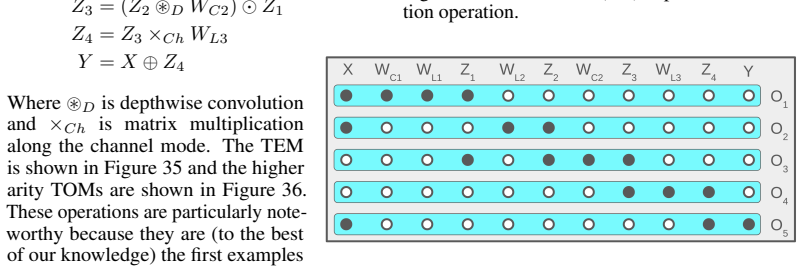
Recognition: unknown
On the Architectural Complexity of Neural Networks
Pith reviewed 2026-05-08 17:26 UTC · model grok-4.3
The pith
A framework that models tensor operations in neural networks shows groundbreaking architectures increase specific types of complexity.
A machine-rendered reading of the paper's core claim, the machinery that carries it, and where it could break.
Core claim
Our study of DNNs introduced over the past 40 years reveals a connection between groundbreaking architectures and increases in different types of architectural complexity. The framework enables two novel objectives: analysis of the evolution of architectural complexity over deep learning history, and automatic construction of novel architectures based on new types of tensor operations. Several large classes of higher complexity architectures have not yet been explored.
What carries the argument
The unified theoretical framework that explicitly models the structure of tensor operations to quantify and generate increases in architectural complexity.
If this is right
- Groundbreaking architectures increase distinct complexity types rather than overall complexity.
- Automatic construction of new architectures becomes feasible by introducing previously unused tensor operations.
- Large families of higher-complexity architectures remain unexplored and can now be enumerated systematically.
- A dataset of over 3,000 higher-complexity architectures is now available for further research and construction.
Where Pith is reading between the lines
- Targeting particular complexity increases could become a design heuristic for creating more capable networks.
- The same tensor-operation lens might be applied to measure complexity growth in non-neural learning systems.
- Empirical tests could check whether the identified complexity jumps reliably predict gains in accuracy or efficiency.
Load-bearing premise
The chosen modeling of tensor operations captures the structural features that actually drive architectural breakthroughs rather than merely correlating with them.
What would settle it
A new neural-network architecture that delivers a clear breakthrough in performance or capability while showing no increase in any of the framework's defined complexity types would falsify the claimed connection.
Figures


read the original abstract
We introduce a unified theoretical framework for the rigorous analysis and systematic construction of deep neural networks (DNNs). This framework addresses a gap in existing theory by explicitly modeling the structure of tensor operations -- lower level information that is often abstracted. Our framework enables two novel objectives: (1) analysis of the evolution of architectural complexity over deep learning history, and (2) automatic construction of novel architectures based on new types of tensor operations. Our study of DNNs introduced over the past 40 years reveals a connection between groundbreaking architectures and increases in different types of architectural complexity. Moreover, we identify several large classes of higher complexity architectures that have not yet been explored. We then collect a dataset of 3,000+ higher complexity architectures, which we publicly release at: https://github.com/combinatoriallabs/ArchitecturalComplexity.
Editorial analysis
A structured set of objections, weighed in public.
Referee Report
Summary. The paper introduces a unified theoretical framework for deep neural networks that explicitly models the structure of tensor operations. This framework is used to analyze the evolution of architectural complexity across DNNs introduced over the past 40 years, revealing a claimed connection between groundbreaking architectures and increases in various complexity types. It further identifies unexplored classes of higher-complexity architectures and releases a public dataset of over 3,000 such architectures.
Significance. If the tensor-operation modeling supplies an independent, a priori complexity metric that can be applied uniformly without hindsight bias, the work could provide a systematic lens on why certain architectures succeeded historically and a basis for generating new ones. The public dataset release is a concrete positive contribution that enables community follow-up.
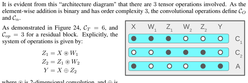
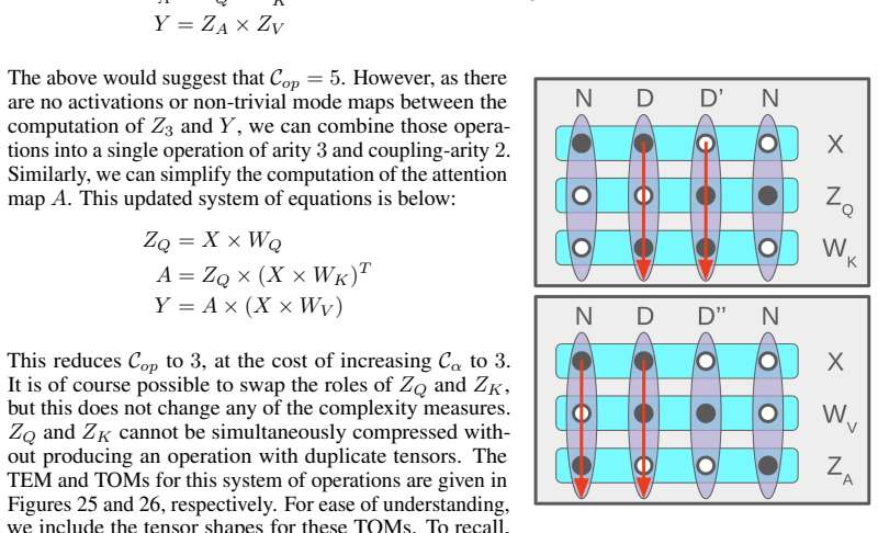
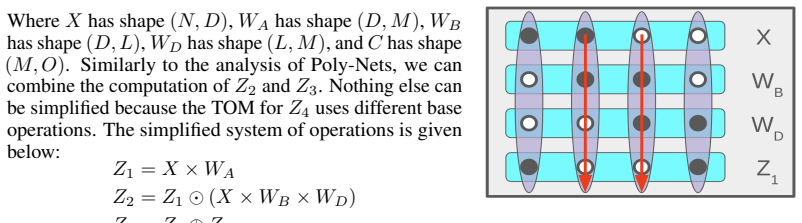
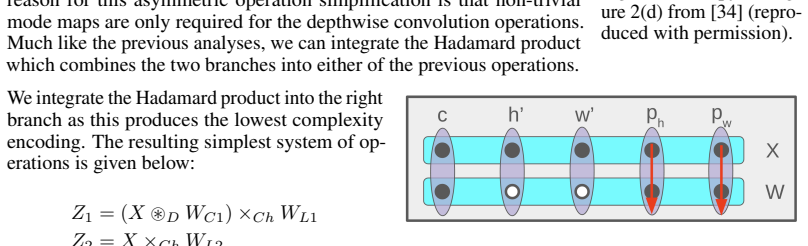
major comments (1)
- The central historical analysis risks circularity: if complexity types are identified by inspecting the tensor operations that distinguish the 'groundbreaking' architectures (e.g., skip connections or attention), then the reported correlation is at least partly definitional rather than predictive. The manuscript must demonstrate that the complexity measures are pre-specified and applied blindly to a fixed corpus, independent of the historical narrative used to select examples.
minor comments (1)
- The abstract and early sections provide only high-level descriptions of the framework and findings; concrete definitions of the complexity types, the precise tensor-operation primitives, and an example calculation on a known architecture (e.g., ResNet or Transformer) would improve accessibility.
Simulated Author's Rebuttal
We thank the referee for their thoughtful and constructive review of our manuscript. We address the single major comment below, and we will revise the paper to improve the clarity of our methodological description.
read point-by-point responses
-
Referee: The central historical analysis risks circularity: if complexity types are identified by inspecting the tensor operations that distinguish the 'groundbreaking' architectures (e.g., skip connections or attention), then the reported correlation is at least partly definitional rather than predictive. The manuscript must demonstrate that the complexity measures are pre-specified and applied blindly to a fixed corpus, independent of the historical narrative used to select examples.
Authors: We appreciate the referee highlighting this methodological concern. The complexity types in our framework (arity, transformation, and composition complexity) are formally defined in Sections 2 and 3 as general mathematical properties of arbitrary tensor operation sequences; these definitions are stated prior to any reference to specific architectures or historical events and make no use of examples such as skip connections or attention. The historical corpus consists of a fixed list of 42 landmark DNNs spanning 1980–2023, compiled from established surveys of deep-learning history and selected solely on the basis of their documented impact in the literature, without reference to our metrics. The pre-defined measures were then applied uniformly to this corpus. We acknowledge that the current manuscript does not contain an explicit statement of this ordering and pre-specification. In the revised version we will therefore insert a new subsection (tentatively 4.1) that (i) restates the a-priori definitions, (ii) reproduces the exact corpus list together with its selection criteria, and (iii) describes the blind computation procedure. This addition will make the independence of the analysis fully transparent. revision: yes
Circularity Check
No significant circularity; framework and historical analysis presented as independent
full rationale
The provided abstract and excerpts introduce a tensor-operation modeling framework as a novel, independent tool for both analyzing 40 years of DNN history and constructing new architectures. The claimed connection between groundbreaking architectures and complexity increases is presented as an empirical revelation from applying the framework, not as a definitional or fitted outcome. No equations, self-citations, or derivations are quoted that reduce the complexity measure to the same operations used to label architectures as groundbreaking. The release of a separate 3000+ architecture dataset further indicates an external corpus. Per hard rules, absent specific quotable reductions (e.g., Eq. X defined in terms of Y or fitted parameter renamed as prediction), the derivation chain is self-contained with no circularity.
Axiom & Free-Parameter Ledger
Reference graph
Works this paper leans on
-
[1]
Martín Abadi, Ashish Agarwal, Paul Barham, Eugene Brevdo, Zhifeng Chen, Craig Citro, Greg S. Corrado, Andy Davis, Jeffrey Dean, Matthieu Devin, Sanjay Ghemawat, Ian Goodfellow, Andrew Harp, Geoffrey Irving, Michael Isard, Yangqing Jia, Rafal Jozefowicz, Lukasz Kaiser, Manjunath Kudlur, Josh Levenberg, Dandelion Mané, Rajat Monga, Sherry Moore, Derek Murra...
2015
-
[2]
Eskue, Roger M
Sasan Salmani Pour Avval, Nathan D. Eskue, Roger M. Groves, and Vahid Yaghoubi. Systematic review on neural architecture search.Artificial Intelligence Review, 2025
2025
-
[3]
Pld: A choice-theoretic list-wise knowledge distillation
Ejafa Bassam, Dawei Zhu, and Kaigui Bian. Pld: A choice-theoretic list-wise knowledge distillation. InNeurIPS, 2025
2025
-
[4]
Alain Bretto.Hypergraph Theory, an Introduction.Springer, 2013. 10
2013
-
[5]
Bronstein, Joan Bruna, Taco Cohen, and Petar Veliˇckovi´c
Michael M. Bronstein, Joan Bruna, Taco Cohen, and Petar Veliˇckovi´c. Geometric deep learning: Grids, groups, graphs, geodesics, and gauges. 2021
2021
-
[6]
Chrysos, Markos Georgopoulos, and V olkan Cevher
Yixin Cheng, Grigorios G. Chrysos, Markos Georgopoulos, and V olkan Cevher. Multilinear operator networks. InICLR, 2024
2024
-
[7]
Chrysos, Stylianos Moschoglou, Giorgos Bouritsas, Yannis Panagakis, Jiankang Deng, and Stefanos Zafeiriou
Grigorios G. Chrysos, Stylianos Moschoglou, Giorgos Bouritsas, Yannis Panagakis, Jiankang Deng, and Stefanos Zafeiriou. P-nets: Deep polynomial neural networks. InCVPR, 2020
2020
-
[8]
Chrysos, Markos Georgopoulos, Jiankang Deng, Jean Kossaifi, Yannis Panagakis, and Anima Anandkumar
Grigorios G. Chrysos, Markos Georgopoulos, Jiankang Deng, Jean Kossaifi, Yannis Panagakis, and Anima Anandkumar. Augmenting deep classifiers with polynomial neural networks. In ECCV, 2022
2022
-
[9]
Chrysos, Yongtao Wu, Razvan Pascanu, Philip H.S
Grigorios G. Chrysos, Yongtao Wu, Razvan Pascanu, Philip H.S. Torr, and V olkan Cevher. Hadamard product in deep learning: Introduction, advances and challenges. InIEEE PAMI, 2025
2025
-
[10]
Deformable convolutional networks
Jifeng Dai, Haozhi Qi, Yuwen Xiong, Yi Li, Guodong Zhang, Han Hu, and Yichen Wei. Deformable convolutional networks. InICCV, 2017
2017
-
[11]
Nas-bench-201: Extending the scope of reproducible neural architecture search
Xuanyi Dong and Yi Yang. Nas-bench-201: Extending the scope of reproducible neural architecture search. InICLR, 2020
2020
-
[12]
An image is worth 16x16 words: Transformers for image recognition at scale
Alexey Dosovitskiy, Lucas Beyer, Alexander Kolesnikov, Dirk Weissenborn, Xiaohua Zhai, Thomas Unterthiner, Mostafa Dehghani, Matthias Minderer, Georg Heigold, Sylvain Gelly, Jakob Uszkoreit, , and Neil Houlsby. An image is worth 16x16 words: Transformers for image recognition at scale. InICLR, 2021
2021
-
[13]
On expressivity and trainability of quadratic networks
Feng-Lei Fan, Mengzhou Li, Fei Wang, Rongjie Lai, and Ge Wang. On expressivity and trainability of quadratic networks. InIEEE NNLS, 2023
2023
-
[14]
Araujo, and Petar Velickovi´c
Bruno Gavranovi´c, Paul Lessard, Andrew Dudzik, Tamara von Glehn, Joao G.M. Araujo, and Petar Velickovi´c. Position: Categorical deep learning is an algebraic theory of all architectures. InICML, 2024
2024
-
[15]
Mamba: Linear-time sequence modeling with selective state spaces,
Albert Gu and Tri Dao. Mamba: Linear-time sequence modeling with selective state spaces,
-
[16]
URLhttps://arxiv.org/abs/2312.00752
work page internal anchor Pith review arXiv
-
[17]
Dey, Soham Mukherjee, Shreyas N
Mustafa Hajij, Ghada Zamzmi, Theodore Papamarkou, Nina Miolane, Aldo Guzmán-Sáenz, Karthikeyan Natesan Ramamurthy, Tolga Birdal, Tamal K. Dey, Soham Mukherjee, Shreyas N. Samaga, Neal Livesay, Robin Walters, Paul Rosen, and Michael T. Schaub. Topological deep learning: Going beyond graph data. 2022
2022
-
[18]
Davenport, Sheik Dawood, Balaji Cherukuri, Joseph G
Mustafa Hajij, Lennart Bastian, Sarah Osentoski, Hardik Kabaria, John L. Davenport, Sheik Dawood, Balaji Cherukuri, Joseph G. Kocheemoolayil, Nastaran Shahmansouri, Adrian Lew, Theodore Papamarkou, and Tolga Birdal. Copresheaf topological neural networks: A general- ized deep learning framework. InNeurIPS, 2025
2025
-
[19]
Deep residual learning for image recognition
Kaiming He, Xiangyu Zhang, Shaoqing Ren, , and Jian Sun. Deep residual learning for image recognition. InCVPR, 2016
2016
-
[20]
Category-theoretical and topos- theoretical frameworks in machine learning: A survey.Axioms, 2025
Yiyang Jia, Guohong Peng, Zheng Yang, and Tianhao Chen. Category-theoretical and topos- theoretical frameworks in machine learning: A survey.Axioms, 2025
2025
-
[21]
On the expressive power of deep polynomial neural networks
Joe Kileel, Matthew Trager, and Joan Bruna. On the expressive power of deep polynomial neural networks. InNeurIPS, 2019
2019
-
[22]
Kingma and J
D. Kingma and J. Ba. Adam: A method for stochastic optimization. InICLR, 2015
2015
-
[23]
Krizhevsky, V
A. Krizhevsky, V . Nair, and G. Hinton. Cifar-10 and cifar100 datasets. 2009. URL https: //www.cs.toronto.edu/kriz/cifar.html
2009
-
[24]
Alex Krizhevsky, Ilya Sutskever, and Geoffrey E. Hinton. Imagenet classification with deep convolutional neural networks. InNeurIPS, 2012. 11
2012
-
[25]
Tiny imagenet visual recognition challenge
Ya Le and Xuan Yang. Tiny imagenet visual recognition challenge. 2015. URL https: //api.semanticscholar.org/CorpusID:16664790
2015
-
[26]
Y . Lecun, L. Bottou, Y . Bengio, and P. Haffner. Gradient-based learning applied to document recognition.Proceedings of the IEEE, 86(11):2278–2324, 1998. doi: 10.1109/5.726791
-
[27]
Diversity-enhanced distribution alignment for dataset distillation
Hongcheng Li, Yucan Zhou, Xiaoyan Gu, Bo Li, and Weiping Wang. Diversity-enhanced distribution alignment for dataset distillation. InICCV, 2025
2025
-
[28]
Darts: Differentiable architecture search
Hanxiao Liu, Karen Simonyan, and Yiming Yang. Darts: Differentiable architecture search. In ICLR, 2019
2019
-
[29]
Swin transformer: Hierarchical vision transformer using shifted windows
Ze Liu, Yutong Lin, Yue Cao, Han Hu, Yixuan Wei, Zheng Zhang, Stephen Lin, and Baining Guo. Swin transformer: Hierarchical vision transformer using shifted windows. InICCV, 2021
2021
-
[30]
Algebra unveils deep learning an invitation to neuroalgebraic geometry
Giovanni Luca Marchetti, Vahid Shahverdi, Stefano Mereta, Matthew Trager, and Kathlen Kohn. Algebra unveils deep learning an invitation to neuroalgebraic geometry. InICML, 2025
2025
-
[31]
Mesner and Prabir Bhattacharya
Dale M. Mesner and Prabir Bhattacharya. Association schemes on triples and a ternary algebra. JOURNAL OF COMBINATORIAL THEORY, 1988
1988
-
[32]
Ibomoiye Domor Mienye and Theo G. Swart. A comprehensive review of deep learning: Architectures, recent advances, and applications. InInformation, 2024
2024
-
[33]
Spiralmlp: A lightweight vision mlp architecture
Haojie Mu, Burhan Ul Tayyab, and Nicholas Chua. Spiralmlp: A lightweight vision mlp architecture. InWACV, 2024
2024
-
[34]
Folding over neural networks, 2022
Minh Nguyen and Nicholas Wu. Folding over neural networks, 2022
2022
-
[35]
Deep tree tensor networks for image recognition
Chang Nie, Junfang Chen, and Yajie Chen. Deep tree tensor networks for image recognition. In NeurIPS, 2025
2025
-
[36]
A survey on state-of-the-art deep learning applications and challenges
Mohd Halim Mohd Noor and Ayokunle Olalekan Ige. A survey on state-of-the-art deep learning applications and challenges. InEngineering Applications of Artificial Intelligence, 2025
2025
-
[37]
Automatic differentiation in pytorch
Adam Paszke, Sam Gross, Soumith Chintala, Gregory Chanan, Edward Yang, Zachary DeVito, Zeming Lin, Alban Desmaison, Luca Antiga, and Adam Lerer. Automatic differentiation in pytorch. InNIPS-W, 2017
2017
-
[38]
Learning representations by back- propagating errors., 1986
David Rumelhart, Geoffrey Hinton, and Ronald Williams. Learning representations by back- propagating errors., 1986
1986
-
[39]
Sandler, A
M. Sandler, A. G. Howard, M. Zhu, A. Zhmoginov, and L. Chen. Mobilenetv2: Inverted residuals and linear bottlenecks. InCVPR, 2018
2018
-
[40]
Learning on a razor’s edge: the singularity bias of polynomial neural networks
Vahid Shahverdi, Giovanni Luca Marchetti, and Kathlen Kohn. Learning on a razor’s edge: the singularity bias of polynomial neural networks. InICLR, 2026
2026
-
[41]
Simonyan and A
K. Simonyan and A. Zisserman. Very deep convolutional networks for large-scale image recognition. InICLR, 2015
2015
-
[42]
Smith and Nicholay Topin
Leslie N. Smith and Nicholay Topin. Super-convergence: Very fast training of neural networks using large learning rates, 2017
2017
-
[43]
Logit standardization in knowledge distillation
Shangquan Sun, Wenqi Ren, Jingzhi Li, Rui Wang, and Xiaochun Cao. Logit standardization in knowledge distillation. InCVPR, 2024
2024
-
[44]
Pure and spurious critical points: A geometric study of linear networks
Matthew Trager, Kathlen Kohn, and Joan Bruna. Pure and spurious critical points: A geometric study of linear networks. InICLR, 2020
2020
-
[45]
Gomez, Lukasz Kaiser, and Illia Polosukhin
Ashish Vaswani, Noam Shazeer, Niki Parmar, Jakob Uszkoreit, Llion Jones, Aidan N. Gomez, Lukasz Kaiser, and Illia Polosukhin. Attention is all you need. InNeurIPS, 2017
2017
-
[46]
Equivariant and coordinate independent convolutional networks, 2023
Maurice Weiler, Patrick Forré, Erik Verlinde, and Max Welling. Equivariant and coordinate independent convolutional networks, 2023. 12
2023
-
[47]
Nas-bench-101: Towards reproducible neural architecture search
Chris Ying, Aaron Klein, Esteban Real, Eric Christiansen, Kevin Murphy, and Frank Hutter. Nas-bench-101: Towards reproducible neural architecture search. InICML, 2019
2019
-
[48]
Arsiwalla, and Taliesin Beynon
Carlos Zapata-Carratalá, Xerxes D. Arsiwalla, and Taliesin Beynon. Diagrammatic calculus and generalized associativity for higher-arity tensor operations.Theoretical Computer Science, 2024
2024
-
[49]
list distances
Lianghui Zhu, Bencheng Liao, Qian Zhang, Xinlong Wang, Wenyu Liu, and Xinggang Wang. Vision mamba: Efficient visual representation learning with bidirectional state space model. In ICML, 2024. 13 Table of Contents ATheoretical Appendix. A.1Generalized Tensors. A.1.1 Technical Background. A.1.2 Complete definition of the slice ordering compatibility condit...
2024
-
[50]
A partition ofE,P∈ P(P(E)). 17
-
[51]
one index away
An edge-indexed family of strict weak orders, <e ⊊e×e e∈E. A PWO-HG without the partition is called aweakly ordered hypergraph. Intuitively, weakly ordered hypergraphs are hypergraphs which have lists for edges. As such, they are a strict generalization of the well-studied interval hypergraphs (see [4], section 4.1). We recall that an interval hypergraph ...
-
[52]
For any pathγ, X p∈P dp(γ) =d(γ)
-
[53]
For any pathγ, d p(γ) =−d p(¯γ)
-
[54]
elements
For any pair of composable pathsγ a,b, γb,c, d p(γb,c ◦γ a,b) =d p(γb,c) +d p(γa,b) Proof. These identities follow immediately from the definition of p-distance and the fact that P is a partition ofE. As PWO-HGs will be used to study hyper-tensors, we now introduce the notion of a path between tuples. Definition A.9.Atupleof a PWO-HG H=⟨V, E,{< e}e∈E, P⟩ ...
-
[55]
The2-cells ofs 3 form a partition of the⊊-maximal elements ofX 1|s3
-
[56]
∀x∈ X 0|s3 ,∃{s 1 i }i∈I ⊏s 3 withx∈ |s3|\ i=1 s1 i
Eachx∈ X 0|s3 is contained in the intersection of some transversal of this partition. ∀x∈ X 0|s3 ,∃{s 1 i }i∈I ⊏s 3 withx∈ |s3|\ i=1 s1 i
-
[57]
essentially
The structure H= X 0|s3 ,X 1|s3 ,X 2|s3 forms a partitioned and weakly ordered hyper- graph which satisfies theslice ordering compatibility conditions: (a)His connected. (b) All tuple cycles onHhave zerop-distance, for eachp∈s 3. 19 The only difference from Definition 4.1 is the specification of condition 1 to the subset-maximal elements of s3, which is n...
-
[58]
Whenevera, b∈ X 0|s3 1 satisfy:d(γ a,b) = 0, add[{a, b}]to eachs 2 ∈s 3
-
[59]
degenerate
Whenevera, b∈ X 0|s3 1 satisfy:|d(γ a,b)|= 1, add[a, b]tos 2 ifd s2(γa,b) = 1, otherwise, add[b, a]tos 2, wheres 2 is the2-cell with|d s2(γa,b)|= 1. The generalized tensor s3 2 produced by this construction is maximal because the added 1-cells ensure the required implications. Furthermore, as none of the added 1-cells introduce cycles of non-zero distance...
-
[60]
We can continue this process until we reach some i such that ds1(γxi,xi+1) = 1 and xi ∈s 1 1 and xi+1 ∈s 1
Analogously, x2 ∈s 1 1 and xn−1 ∈s 1 2, and so on. We can continue this process until we reach some i such that ds1(γxi,xi+1) = 1 and xi ∈s 1 1 and xi+1 ∈s 1
-
[61]
efficient
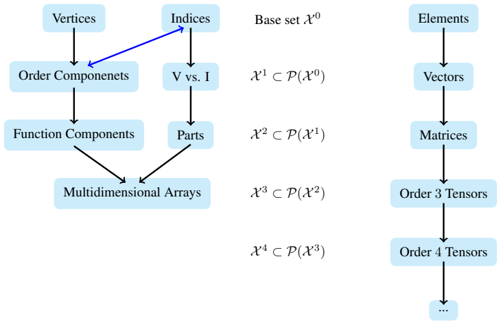
By the previous argument, this is impossible. We conclude thats 3 c is unique up to mode permutations. Canonical representatives are useful for reducing the rank complexity of the HCC encodings of generalized tensors. 23 Vertices Base setX 0 Edges X 1 ⊂ P(X 0) Ordered Pairs X 2 ⊂ P(X 1) Ordered Edges X 3 ⊂ P(X 2) Parts X 4 ⊂ P(X 3) PWO-HGs X 5 ⊂ P(X 4) El...
-
[62]
minor technical update
For each transversal{s 1 i }i∈I ⊏s 3,we have that |s3|\ i=1 s1 i ≤1 thens 3 can be represented as an injective multidimensional array. The “minor technical update” as compared to Theorem 4.2 is the restriction of hypotheses 1 to the canonical representative for s3. This is necessary because hypothesis 1 (theequal lengthcondition) is meaningless in the pre...
-
[63]
exterior corner
Each{v} ∈ X 0 is contained in a transversal of this supposed partition. 3.X 1 satisfies the slice ordering compatibility conditions. To show 1, let s1 ∈ X 1 be a ⊊-maximal 1-cell. By construction, s1 is a set of v∈V which corresponds under T to a set of multi-indices with O−1 of the entries fixed. Let i denote the free index. As X 2 was constructed such t...
-
[64]
That is, pick zi = argmaxz minx∈X 0|Ti d(z, x)
Let Hi be the PWO-HG (Definition A.4) associated to Ti, and pick an origin zi ∈ X 0|Ti to maximize the minimum distance path from zi. That is, pick zi = argmaxz minx∈X 0|Ti d(z, x)
-
[65]
Construct multi-indices for each tuple ofH i with Lemma A.13, setting the origin toz i
-
[66]
Call the resulting set of multi-indices Ii ⊆[[M i,1]]×...×[[M i,Oi]], whereO i =|X 2|Ti |andM i,j is the tensor length of thej th mode ofT i
If necessary, introduce offsets to these indices to ensure that no multi-index contains any non-positive entries. Call the resulting set of multi-indices Ii ⊆[[M i,1]]×...×[[M i,Oi]], whereO i =|X 2|Ti |andM i,j is the tensor length of thej th mode ofT i. 35
-
[67]
Otherwise, assign ∅
Define a Vi-valued multidimensional array Ti by assigning to each multi-index of Ii the corresponding tuple if one exists. Otherwise, assign ∅. By the SOCCs, this is a well-defined function
-
[68]
tensor operation
Collapse the tuples of Ti to their products with the rule: t∈image(T i)7→ Q x∈t x, whereQ is shorthand for iterated application of⋆. This process produces a multidimensional array Ti : [[Mi,1]]×...×[[M i,Oi]]→V i for each tensor Ti. While these multidimensional arrays may be jagged, they are by construction not hyper. Step 2.Denote by M the set of all mod...
-
[69]
Before we discuss the somewhat technical proof, we provide a fundamental corollary as further motivation
Each operand ofs 4 can be represented as an injective multidimensional array 2.⋆distributes over⋄ 3.⋄is associative then, after evaluation using ⋆ and ⋄, s4 is equal to the composition of an (α−1) -arity tensor operation and a binary tensor operation. Before we discuss the somewhat technical proof, we provide a fundamental corollary as further motivation....
-
[70]
index" and “mode
To facilitate this process, we now perform some index management: (i1, ..., iσ)— non-contracted indices ofA (iσ+1, ..., iCO)— contracted indices ofA (j1, ..., jρ)— non-contracted indices ofT β froms 4 1 (jρ+1, ..., jOβ)— contracted indices ofT β froms 4 1 (k1, ..., kϱ)— non-contracted indices ofT α ins 4 2 (kϱ+1, ..., kOα)— contracted indices ofT α ins 4 ...
-
[71]
Figure 16: Index map
∆ is non-negative because we only (possibly) removed contractions in the creation ofs 4 1. Figure 16: Index map. Dotted boxes are contracted modes. Next, observe that for each contrac- tion removed in the creation of s4 1, there must exist some k index which is part of the corresponding coupling. This is because of how C1 is defined. Dually, for each cont...
-
[72]
The complete system of index equivalences is given below: (i1, ..., im) = (k1, ..., kϱ) (j1, ..., jm−n) = (kn, ..., kϱ) (j1, ..., jρ) = (in, ..., iσ+∆) (iσ+1, ..., iσ+∆) = (kϱ+1, ..., kϱ+∆) (jρ+1, ..., jOβ) = (iσ+∆+1, ..., iCO−p) Let [[M ′ n]]×..×[[M ′ n+ρ]] be the multi-index set defined by the non-contracted modes of A1, where A1 is the hyper-tensor def...
-
[73]
α−1Y a=1 A1[j1 :j Oβ] [a] # = X (jρ+1:jOβ )
From here on, we write (i1 :i n) as shorthand for (i1, ..., in). We can now evaluates4 1: Tβ : [[M ′ n]]×..×[[M ′ n+ρ]]→F (j1 :j ρ) = (in :i σ+∆)7→ X (jρ+1:jOβ ) " α−1Y a=1 A1[j1 :j Oβ] [a] # = X (jρ+1:jOβ ) " α−1Y a=1 A[∅=i 1 :i n−1, j1 :j Oβ , iσ+∆+1 :i CO =∅] [a] # (5) Here we have used an empty index to indicate broadcasting, i.e., indexing into dummy...
-
[74]
Then, s4 1 and s4 2 can be combined into an equivalent tensor operation of arityα+α ′ −1. Proof. These hypotheses are simply a restatement of the properties satisfied by the tensor operations s4 1 and s4 2 constructed in the proof of Theorem A.35. Therefore, they are equivalent to the tensor operation defined by: s4 :={T∈s 4 1 :Tis a tensor} ∪ {T∈s 4 2 \T...
-
[75]
operand factored
The tensor lengths align by assumption. 41 A.2.4 Additional Examples of Tensor Operations We now provide more examples of tensor operations to facilitate understanding of the main paper. Throughout this section, we assume that F=R , and that the base operations of all tensor operations are real number multiplication and addition. Jagged Matrix Multiplicat...
-
[76]
compli- cated
use compatible base operations with the linear transformations of the CNM. It is interesting to observe that the copresheaf framework is effectively a categorical language for the description of TEMs similar to that of Figure 22. An important detail is that the transformations that can be implemented in a CNM are strictly linear, meaning that in particula...
2017
discussion (0)
Sign in with ORCID, Apple, or X to comment. Anyone can read and Pith papers without signing in.