FAB: A First-Order AB-based Gradient Algorithm for Distributed Bilevel Optimization over Time-Varying Directed Graphs
Pith reviewed 2026-05-08 08:22 UTC · model grok-4.3
The pith
A first-order algorithm integrates Push-Pull communication with value-function penalties to solve distributed bilevel optimization over time-varying directed graphs.
A machine-rendered reading of the paper's core claim, the machinery that carries it, and where it could break.
Core claim
The central claim is that the FAB algorithm, formed by embedding the Push-Pull communication protocol inside a value-function-based penalty framework, converges at a non-asymptotic rate to stationary points of the distributed bilevel problem over time-varying directed graphs, while a simplified version of the same analysis yields an explicit rate for Push-Pull in the nonconvex single-level case.
What carries the argument
The integration of the Push-Pull (AB) strategy, which maintains two separate weight sequences to achieve consensus on unbalanced directed graphs, with a value-function penalty that converts the bilevel structure into a single penalized objective.
If this is right
- The method directly applies to distributed hyperparameter tuning and data hyper-cleaning without requiring second-order derivatives or centralized coordination.
- It supplies the first explicit convergence rate for the Push-Pull algorithm on nonconvex single-level problems over time-varying directed graphs.
- The same analysis framework can be reused to derive rates for other first-order distributed methods that handle nested objectives.
- Practical tasks such as distributed reinforcement learning become feasible on dynamic networks with the same communication cost as single-level methods.
Where Pith is reading between the lines
- The value-function penalty may extend to other nested optimization structures beyond bilevel problems in multi-agent systems.
- The approach suggests that similar penalty reductions could simplify analysis of federated bilevel learning under changing topologies.
- Further work could test whether the same rates hold when communication is stochastic or when agents use asynchronous updates.
- The resolved open question on Push-Pull rates opens the door to using that protocol as a building block for more complex distributed learning tasks.
Load-bearing premise
The sequence of directed graphs must satisfy joint connectivity and balance conditions over time so that consensus is eventually reached despite individual graphs being unbalanced and time-varying.
What would settle it
Numerical runs of the algorithm on a periodic sequence of directed graphs whose union graph is not strongly connected, checking whether the iterates fail to approach any stationary point of the bilevel problem.
Figures


read the original abstract
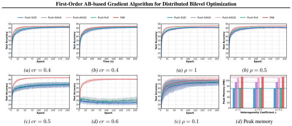
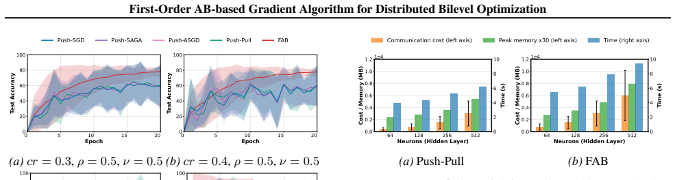
Distributed optimization over time-varying directed graphs has shown promising performance in addressing challenges posed by complex communication constraints in real-world scenarios. In many practical settings, however, the direct application of distributed optimization algorithms encounters additional difficulties, most notably hyperparameter tuning, which our empirical observations suggest can be effectively mitigated by integrating bilevel optimization. Motivated by these findings, we study distributed bilevel optimization over time-varying directed networks, a problem that remains largely unexplored due to the compounded challenges arising from consensus bias in dynamic unbalanced communication and the nested optimization structure. In this work, we propose a fully first-order distributed gradient-based algorithm that integrates the Push-Pull (also known as AB) communication strategy with a value function-based penalty method and establish its non-asymptotic convergence properties. Notably, a simplified variant of our analysis framework for nonconvex single-level distributed optimization establishes a convergence rate for the Push-Pull algorithm, thereby resolving an open question concerning its convergence over time-varying directed graphs. Empirical evaluations across diverse tasks, including hyperparameter tuning, data hyper-cleaning, and reinforcement learning, validate the effectiveness and efficiency of the proposed algorithm.
Editorial analysis
A structured set of objections, weighed in public.
Referee Report
Summary. The paper introduces the FAB algorithm for distributed bilevel optimization over time-varying directed graphs. It combines the Push-Pull (AB) strategy with a value function-based penalty method to create a fully first-order distributed gradient-based algorithm. The authors establish non-asymptotic convergence properties for this algorithm. A simplified analysis framework is used to provide a convergence rate for the Push-Pull algorithm in the context of nonconvex single-level distributed optimization, thereby addressing an open question regarding its convergence over time-varying directed graphs. The approach is validated through empirical studies on hyperparameter tuning, data hyper-cleaning, and reinforcement learning tasks.
Significance. If the claimed non-asymptotic convergence rates hold under the stated assumptions, this work would make a notable contribution to distributed optimization by providing the first such guarantees for bilevel problems on time-varying directed graphs and resolving the open question on Push-Pull convergence. The integration of bilevel optimization to mitigate hyperparameter tuning issues is practically relevant. The first-order nature and handling of unbalanced dynamic networks are strengths. The empirical validation across diverse tasks supports the practical utility.
minor comments (2)
- [Abstract] The abstract asserts non-asymptotic convergence without providing a proof sketch or explicit assumptions; while the full manuscript likely contains these, a brief mention could improve accessibility.
- [Empirical Evaluations] The experiments validate the algorithm but could include more details on the graph topologies used to demonstrate the time-varying directed nature.
Simulated Author's Rebuttal
We thank the referee for the positive review, the recognition of our contributions to distributed bilevel optimization over time-varying directed graphs, and the recommendation for minor revision. We are pleased that the work's novelty in providing non-asymptotic convergence guarantees and resolving the open question on Push-Pull convergence has been acknowledged.
Circularity Check
No significant circularity; derivation self-contained
full rationale
The paper introduces a novel first-order algorithm combining the established Push-Pull (AB) strategy with a value-function penalty for distributed bilevel optimization over time-varying directed graphs, then derives non-asymptotic convergence under standard smoothness and connectivity assumptions. A simplified variant of this analysis is used to obtain a rate for single-level nonconvex Push-Pull, presented as resolving an open question. No step reduces by construction to a fitted parameter, self-definition, or load-bearing self-citation chain; the central claims rest on fresh analysis rather than renaming or smuggling prior results. The derivation is therefore self-contained against external benchmarks.
Axiom & Free-Parameter Ledger
free parameters (1)
- step sizes and penalty parameter
axioms (2)
- domain assumption Time-varying directed graphs satisfy connectivity and balance conditions sufficient for consensus despite being unbalanced and dynamic.
- domain assumption Objective functions are sufficiently smooth and satisfy standard assumptions for bilevel optimization.
Reference graph
Works this paper leans on
-
[1]
Xin, R., Pu, S., Nedi ´c, A., and Khan, U
IEEE, 2019. Xin, R., Pu, S., Nedi ´c, A., and Khan, U. A. A general framework for decentralized optimization with first-order methods.Proceedings of the IEEE, 108(11):1869–1889, 2020. Yang, S., Zhang, X., and Wang, M. Decentralized gossip- based stochastic bilevel optimization over communication networks. InAdvances in Neural Information Processing System...
work page 2019
-
[2]
Network and setup:The system comprises n= 10 agents connected via a default topology
To perform binary classification, we append a linear classification head to the output representations of the backbone, mapping the extracted features to the2sentiment classes. Network and setup:The system comprises n= 10 agents connected via a default topology. We vary the connection probability ν∈ {0.1,0.5} . The dataset is partitioned using a Dirichlet...
work page 2023
-
[3]
Contraction of the unregularized estimatorˆzk: ˆzk+1 −y ∗(ˆxk+1) 2 ≤(1 +δ k,1) " (1 +δ k,2)qz,k(ηk z ) ˆzk −y ∗(ˆxk) 2 + 1 + 1 δk,2 (ηk z )2 2S(tk z , βk) + 6λ2L2 g,1 n min(αk) Vk D # + L2 g,1 µ2 1 + 1 δk,1 ˆxk+1 −ˆxk 2 .(42)
-
[4]
Contraction of the regularized estimatorˆyk: ˆyk+1 −y ∗ λ(ˆxk+1) 2 ≤(1 +δ k,3) " (1 +δ k,4)qy,k(ηk y) ˆyk −y ∗ λ(ˆxk) 2 + 1 + 1 δk,4 (ηk y)2 2S(tk y, βk) + 8(L2 f,1 +λ 2L2 g,1) n min(αk) Vk D # + 9L2 g,1 µ2 1 + 1 δk,3 ˆxk+1 −ˆxk 2 .(43) where Vk D is defined in (30), S(tk ξ , βk) is defined in (29). The weight vectors αk and βk are specified in Lemmas D.4...
work page 2018
-
[5]
The consensus of tracking variables: We must verify that the auxiliary tracking variables accurately estimate the global gradients (i.e.,S→0). In this section, we derive the recurrence relationships for these quantities, showing that they contract linearly up to a perturbation term controlled by the step sizes. We define thestacked weighted average vector...
work page 2025
-
[6]
Coefficient of the drift term ∥ˆxk+1 −ˆxk∥2.Collecting all terms involving the decision variable difference, we obtain the coefficient: C(b) Φ,1 =− 1 α β 1 2ηkx + L∗,1 2 +C b,1 2L2 g,1 ληkz q βµ2 +C b,2 72L2 g,1 ληky q βµ2
-
[7]
40 First-Order AB-based Gradient Algorithm for Distributed Bilevel Optimization
Coefficient of the unregularized estimation error∥ˆzk −y ∗(ˆxk)∥2.Grouping the terms associated with the lower-level variablez, the coefficient is: C(b) Φ,2 = ηk x 2 6λ2L2 g,1n2α2β αβ −C b,1ληk z q β + 2 c Cb,3α βη k x 2 + 56Cb,4 γ e λ2L2 g,13ηk x 2 4n2λ2L2 g,1 + 2 c Cb,3α βη k z 2 + 56Cb,4 γ e λ2L2 g,13ηk z 2 2n2λ2L2 g,1. 40 First-Order AB-based Gradient...
-
[8]
Coefficient of the regularized estimation error∥ˆyk −y ∗ λ(ˆxk)∥2.Similarly, for the variabley, the coefficient is: C(b) Φ,3 = 12ηk xλ2L2 g,1n2α2β αβ −C b,2ληk y q β + 2 c Cb,3α βη k x 2 + 56Cb,4 γ e λ2L2 g,13ηk x 2 4n2λ2L2 g,1 + 2 c Cb,3α βη k y 2 + 56Cb,4 γ e λ2L2 g,13ηk y 2 8n2λ2L2 g,1
-
[9]
Coefficient of the consensus error n α Vk D.The coefficient for the consensus error consists of the negative contraction term from the graph topology and positive perturbations: C(b) Φ,4 = 1 α β 18λ2L2 g,1 ηk x 2 +C b,1 12 λq β ηk z λ2L2 g,1 +C b,2 32 λq β ηk y λ2L2 g,1 −C b,3c + 336Cb,4 γ e λ2L2 g,1 + 2 c Cb,3α β+ 168C b,4 γ e λ2L2 g,1 36λ2L2 g,1(ηk x 2 ...
-
[10]
Coefficient of the tracking errorV k S.The coefficient for the gradient tracking error is: C(b) Φ,5 = 3 α β ηk x +C b,1 4 λq β ηk z +C b,2 4 λq β ηk y −C b,4e + 2 c Cb,3α β+ 168C b,4 γ e λ2L2 g,1 (ηk x 2 +η k y 2 +η k z 2 )
-
[11]
Coefficient of the gradient norm∥∇ xL∗ λ(ˆxk)∥2.Finally, the coefficient for the descent term is: C(b) Φ,6 = 2 c Cb,3α β+ 168C b,4 γ e λ2L2 g,1 4n2ηk x 2 − ηk x 2 α β. By ensuring that the step-sizes and the penalty parameter λ satisfy conditions (79)–(81), we guarantee that the coefficients C(b) Φ,1, C(b) Φ,2, C(b) Φ,3, and C(b) Φ,5 are non-positive, whi...
work page 2018
-
[12]
Term∥ˆxk+1 −ˆxk∥2: The coefficient is C(s) Φ,1 :=− 1 2ηkxαβ + Lf,1 2
-
[13]
46 First-Order AB-based Gradient Algorithm for Distributed Bilevel Optimization
TermD(x k, αk): The coefficient is C(s) Φ,2 := 3L2 f,1n βα2 ηk x − Cs,1c n α +C s,2 24γL2 f,1 e α + Cs,1 2 c αβ n α +C s,2 12γL2 f,1 e ! 12nL2 f,1 α (ηk x)2. 46 First-Order AB-based Gradient Algorithm for Distributed Bilevel Optimization
-
[14]
TermS(t k x, βk): The coefficient is C(s) Φ,3 := 3 αβ ηk x − Cs,2e +C s,1 2 c (ηk x)2αβ n α +C s,2 12γL2 f,1 e (ηk x)2
-
[15]
Term∥∇ xF(ˆxk)∥2: The coefficient is C(s) Φ,4 :=− αβ 2 ηk x + Cs,1 2 c αβ n α +C s,2 12γL2 f,1 e ! 4n2(ηk x)2. Under these conditions in (103), the coefficients simplify to the desired bounds, yielding: Φ(s)(ˆxk+1)−Φ (s)(ˆxk)≤ − ηk x 4 αβ ∇xF(ˆxk) 2 − Cs,1c 4 n α D(xk, αk).(105) Convergence rate of Push-Pull Theorem E.7.Suppose that Assumptions 3.1 and 3....
discussion (0)
Sign in with ORCID, Apple, or X to comment. Anyone can read and Pith papers without signing in.