Recognition: unknown
When is Warmstarting Effective for Scaling Language Models?
Pith reviewed 2026-05-14 19:56 UTC · model grok-4.3
The pith
A 2x growth factor from smaller checkpoints reliably speeds language model convergence, but an upper bound on growth factor makes training from scratch more efficient beyond it.
A machine-rendered reading of the paper's core claim, the machinery that carries it, and where it could break.
Core claim
Model growth from a given checkpoint accelerates training of a larger model only up to an empirically identified upper bound on the growth factor g, beyond which training from scratch becomes more efficient. Simple, architecture-agnostic growth operators outperform more complex ones that try to preserve the base model's post-growth performance. Across dense MLPs and language models, a 2x growth factor proves most reliable for convergence speedups, with the largest gains under 20 tokens per parameter and diminishing returns at higher budgets. Scaling laws fitted to the observations supply predictive guidance on when and how much to grow.
What carries the argument
The growth factor g that sets the size ratio between base and target model, together with the choice of simple weight-mapping operator that transfers parameters from the smaller checkpoint to the larger one.
If this is right
- A 2x growth factor produces the most reliable convergence speedups across tested setups.
- Speedup gains are largest when the training budget stays below 20 tokens per parameter and shrink as the budget grows.
- Beyond the identified upper bound on growth factor g, training from scratch uses fewer total resources.
- Simple growth operators achieve final performance equal to or better than complex operators that preserve initial performance.
- Fitted scaling laws give practitioners a way to predict whether growth will help at a given model size and budget.
Where Pith is reading between the lines
- The same growth-factor bound may need re-measurement when moving from dense models to sparse or mixture-of-experts architectures.
- Growth could be tested as a way to warm-start early checkpoints in very long pre-training runs rather than only at the start.
- The scaling laws could be used to decide growth points dynamically during a single long training run.
- Replicating the upper-bound finding on public checkpoints would let practitioners apply the guideline without new experiments.
Load-bearing premise
The upper bound on growth factor and the advantage of simple operators will continue to hold for architectures and training regimes beyond the dense MLPs and language models examined here.
What would settle it
A single training run on a transformer or other architecture at a fixed budget where growth factors larger than the reported bound still converge faster than training from scratch would falsify the claimed limit.
Figures


read the original abstract
Model growth from a given checkpoint aims to accelerate training of a larger model, offering potential resource savings. Despite recent interest, warmstarting has seen limited practical adoption in large-scale training. We attribute this to two underexplored factors: (1) an overemphasis on preserving the smaller model's performance at initialization, which constrains operator design for new architectures, and (2) insufficient analysis of how growth interacts with hyperparameters and scaling behavior, compounded by inconsistent growth factors across the literature. We show that preserving the base model's initial post-growth performance is not necessary for strong final performance, and that simple, architecture-agnostic growth strategies can outperform more complex warmstarting operators. Crucially, we empirically identify an upper bound on the growth factor $g$ beyond which training from scratch is more efficient. We observe this across multiple ablation setups. Notably, this limit is also present, but unreported, in prior published results. Across our experiments on dense MLPs and dense language models, we find that a $2\times$ growth factor is the most reliable in yielding convergence speedups, with gains most pronounced under 20 tokens/parameter budgets and diminishing as budget increases. We fit scaling laws over these observations to provide predictive guidance for practitioners deciding when and how much to grow. Together, our analysis provides practical guidelines and empirical limits for model growth.
Editorial analysis
A structured set of objections, weighed in public.
Referee Report
Summary. The paper examines the effectiveness of warmstarting via model growth for scaling dense MLPs and language models. It argues that preserving the base model's post-growth performance is unnecessary for good final results, that simple architecture-agnostic growth operators can outperform complex ones, and that there exists an empirically observed upper bound on the growth factor g beyond which training from scratch is more efficient under fixed token budgets. The work identifies 2x growth as most reliable for convergence speedups (especially below 20 tokens/parameter), with diminishing returns at higher budgets, and fits scaling laws to these observations to offer predictive guidance for practitioners.
Significance. If the central empirical claims hold after addressing hyperparameter interactions, the results would provide actionable limits and guidelines for when warmstarting yields net savings in large-scale training. The scaling-law fits and cross-setup consistency (including unreported patterns in prior work) could help practitioners decide growth factors without exhaustive search, addressing a practical gap in current scaling practice.
major comments (3)
- [Abstract and experimental sections] Abstract and experimental sections: The upper bound on growth factor g (beyond which scratch training wins) is derived under a fixed learning-rate schedule. Given the abstract's own statement that growth-HP interactions have received insufficient prior analysis, it remains possible that re-tuning the LR or schedule for larger g would shift the reported crossover point, weakening the claim that the bound is a general limit rather than an artifact of the chosen regime.
- [Scaling-law fits] Scaling-law fits: The manuscript fits scaling laws to the observed speedups and upper-bound behavior but provides no details on the functional form, fitting procedure, confidence intervals, or out-of-sample validation. Without these, it is difficult to assess whether the laws reliably predict the 2x optimum or the g upper bound for new budgets or architectures.
- [Ablation setups] Ablation setups: The claim that simple growth operators outperform complex ones rests on multiple ablations, yet the abstract and review note the absence of error bars, exact dataset sizes, and precise determination of the upper bound. This leaves open the possibility of post-hoc selection effects in identifying the bound across setups.
minor comments (2)
- [Figures] Figures showing convergence curves should include error bars or multiple random seeds to support the reported speedups and the location of the g upper bound.
- [Experimental details] The manuscript should clarify the exact token budgets and model sizes used in each ablation so readers can reproduce the 20 tokens/parameter threshold.
Simulated Author's Rebuttal
We thank the referee for their constructive comments, which have helped improve the clarity and rigor of the manuscript. We address each major point below and indicate the revisions made.
read point-by-point responses
-
Referee: [Abstract and experimental sections] The upper bound on growth factor g (beyond which scratch training wins) is derived under a fixed learning-rate schedule. Given the abstract's own statement that growth-HP interactions have received insufficient prior analysis, it remains possible that re-tuning the LR or schedule for larger g would shift the reported crossover point, weakening the claim that the bound is a general limit rather than an artifact of the chosen regime.
Authors: We agree that the reported upper bound on g was obtained under a fixed cosine learning-rate schedule with constant peak LR. As noted in the abstract, growth-HP interactions remain underexplored. In the revision we added a sensitivity study (new Figure 7 and Section 4.3) in which peak LR was scaled proportionally with model size for g=4 and g=8; the crossover point where scratch training overtakes growth remains between g=3 and g=4 under the token budgets examined. We have clarified in the abstract and discussion that the bound is observed under standard training regimes while acknowledging that exhaustive per-g hyperparameter search could modestly extend the effective range of g. revision: partial
-
Referee: [Scaling-law fits] The manuscript fits scaling laws to the observed speedups and upper-bound behavior but provides no details on the functional form, fitting procedure, confidence intervals, or out-of-sample validation. Without these, it is difficult to assess whether the laws reliably predict the 2x optimum or the g upper bound for new budgets or architectures.
Authors: We have expanded Appendix C with the precise functional form (a modified Kaplan et al. (2020) law that includes g as an additional covariate), the nonlinear least-squares fitting procedure performed on log-loss, bootstrap-derived 95% confidence intervals, and out-of-sample R^2 results on two held-out token budgets (R^2 > 0.94). These additions confirm that the fitted laws reliably recover the 2x optimum and the observed upper bound on g. revision: yes
-
Referee: [Ablation setups] The claim that simple growth operators outperform complex ones rests on multiple ablations, yet the abstract and review note the absence of error bars, exact dataset sizes, and precise determination of the upper bound. This leaves open the possibility of post-hoc selection effects in identifying the bound across setups.
Authors: All ablation figures now display error bars (standard deviation over three random seeds). Exact dataset sizes and token budgets are stated explicitly in Section 3 (5 B tokens for MLP ablations, 20 B tokens for language-model runs). The upper-bound determination procedure is formalized in new Appendix B: scaling laws are fit independently per setup and the crossover g is computed where predicted growth loss equals scratch loss. This data-driven definition yields a consistent bound across setups and reduces post-hoc selection concerns. revision: yes
Circularity Check
Empirical scaling-law fits on growth experiments; no derivation reduces to inputs by construction
full rationale
The paper performs ablation experiments across dense MLPs and language models, observes an upper bound on growth factor g, and fits scaling laws to those observations for predictive guidance. This is standard empirical practice: the scaling laws are fitted post-experiment to summarize trends rather than being presupposed in the experimental design or claimed as first-principles derivations. No self-definitional equations, fitted-input predictions, or load-bearing self-citations appear in the abstract or described chain. The upper-bound claim is presented as a newly noted pattern across setups (including re-analysis of prior work), not as a mathematical necessity derived from the authors' own prior theorems. Minor self-citation risk exists in any AutoML-adjacent field but is not load-bearing here.
Axiom & Free-Parameter Ledger
free parameters (1)
- growth factor g
Reference graph
Works this paper leans on
-
[1]
S. Bergsma, B. C. Zhang, N. Dey, S. Muhammad, G. Gosal, and J. Hestness. Scaling with collapse: Efficient and predictable training of llm families.arXiv preprint arXiv:2509.25087,
-
[2]
T. Brown, B. Mann, N. Ryder, M. Subbiah, J. Kaplan, P. Dhariwal, A. Neelakantan, P. Shyam, G. Sastry, A. Askell, S. Agarwal, A. Herbert-V oss, G. Krueger, T. Henighan, R. Child, A. Ramesh, D. Ziegler, J. Wu, C. Winter, C. Hesse, M. Chen, E. Sigler, M. Litwin, S. Gray, B. Chess, J. Clark, C. Berner, S. McCandlish, A. Radford, I. Sutskever, and D. Amodei. L...
work page 1901
-
[3]
URLhttps://clarelyle.com/posts/2025-06-30-plasticity-norm.html. P. Clark, I. Cowhey, O. Etzioni, T. Khot, A. Sabharwal, C. Schoenick, and O. Tafjord. Think you have solved question answering? try ARC, the AI2 reasoning challenge.arXiv preprint arXiv:1803.05457,
work page internal anchor Pith review Pith/arXiv arXiv 2025
- [4]
- [5]
- [6]
-
[7]
Practical efficiency of muon for pretraining.arXiv preprint arXiv:2505.02222, 2025
Essential AI et al. Practical efficiency of muon for pretraining.arXiv preprint arXiv:2505.02222,
- [8]
-
[9]
O. Filatov, J. Wang, J. Ebert, and S. Kesselheim. Optimal scaling needs optimal norm.arXiv preprint arXiv:2510.03871,
-
[10]
Mamba: Linear-Time Sequence Modeling with Selective State Spaces
A. Gu and T. Dao. Mamba: Linear time sequence modeling with selective state spaces. arXiv:2312.00752 [cs.LG],
work page internal anchor Pith review Pith/arXiv arXiv
-
[11]
Scaling Laws for Neural Language Models
J. Kaplan, S. McCandlish, T. Henighan, T. Brown, B. Chess, R. Child, S. Gray, A. Radford, J. Wu, and D. Amodei. Scaling laws for neural language models.arXiv:2001.08361 [cs.LG],
work page internal anchor Pith review Pith/arXiv arXiv 2001
- [12]
- [13]
- [14]
-
[15]
T. Mihaylov, P. Clark, T. Khot, and A. Sabharwal. Can a suit of armor conduct electricity? a new dataset for open book question answering. InProceedings of the 2018 Conference on Empirical Methods in Natural Language Processing, pages 2381–2391,
work page 2018
-
[16]
URLhttps://arxiv.org/abs/2303.08774. T. Pethick, W. Xie, K. Antonakopoulos, Z. Zhu, A. Silveti-Falls, and V . Cevher. Training deep learning models with norm-constrained lmos. In A. Singh, M. Fazel, D. Hsu, S. Lacoste-Julien, F. Berkenkamp, T. Maharaj, K. Wagstaff, and J. Zhu, editors,Proceedings of the 42nd International Conference on Machine Learning (I...
work page internal anchor Pith review Pith/arXiv arXiv
- [17]
- [18]
-
[19]
J. W. Rae, S. Borgeaud, T. Cai, K. Millican, J. Hoffmann, F. Song, J. Aslanides, S. Henderson, R. Ring, S. Young, et al. Scaling language models: Methods, analysis & insights from training gopher.arXiv preprint arXiv:2112.11446,
work page internal anchor Pith review Pith/arXiv arXiv
-
[20]
M. Samragh, I. Mirzadeh, K. A. Vahid, F. Faghri, M. Cho, M. Nabi, D. Naik, and M. Farajtabar. Scaling Smart: Accelerating large language model pre-training with small model initialization. arXiv:2409.12903 [cs.CL],
-
[21]
B. Shin, J. Oh, H. Cho, and C. Yun. Dash: Warm-starting neural network training without loss of plasticity under stationarity. In R. Salakhutdinov, Z. Kolter, K. Heller, A. Weller, N. Oliver, J. Scarlett, and F. Berkenkamp, editors,2nd Workshop on Advancing Neural Network Training: Computational Efficiency, Scalability, and Resource Optimization (WANT@ IC...
work page 2024
-
[22]
J. Su, Y . Lu, S. Pan, A. Murtadha, B. Wen, and Y . Liu. Roformer: Enhanced transformer with rotary position embedding.arXiv:2104.09864 [cs.CL],
work page internal anchor Pith review Pith/arXiv arXiv
-
[23]
B. Thérien, C. Joseph, B. Knyazev, E. Oyallon, I. Rish, and E. Belilovsky. µlo: Compute-efficient meta-generalization of learned optimizers.arXiv preprint arXiv:2406.00153,
-
[24]
LLaMA: Open and Efficient Foundation Language Models
H. Touvron, T. Lavril, G. Izacard, X. Martinet, M. Lachaux, T. Lacroix, B. Rozière, N. Goyal, E. Hambro, F. Azhar, A. Rodriguez, A. Joulin, E. Grave, and G. Lample. LLaMA: Open and efficient foundation language models.arXiv preprint arXiv:2302.13971,
work page internal anchor Pith review Pith/arXiv arXiv
-
[25]
14 E. Unlu. Preservation is not enough for width growth: Regime-sensitive selection of dense lm warm starts.arXiv preprint arXiv:2604.04281,
work page internal anchor Pith review Pith/arXiv arXiv
- [26]
- [27]
-
[28]
15 A Supporting Related Work Scaled parameterizationsrefer to a set of rules that determine how certain parameters can be scaled with respect to one or more scaling dimensions [Everett et al., 2024]. This family of parameteriza- tions describes scaling factors for the weights, the learning rate, and the standard deviation of the initialization. Each of th...
work page 2024
-
[29]
look at how µP, collapsed scaling curves, and novel parametric forms for scaling relationships together can be leveraged for early stopping learning curves. B Synthetic Regression Benchmark We use the synthetic regression benchmark in which the target function is constructed to have a power-law Fourier spectrum [Qiu et al., 2025]. Following their compute ...
work page 2025
-
[30]
Grid Sizes.The base grid contains 8·3·5·3·2 = 720 configurations
are over thefull grid at the target width. Grid Sizes.The base grid contains 8·3·5·3·2 = 720 configurations. The main grid contains 4·3·3·3·2 = 216 configurations. Unless stated otherwise, each experimental setting uses the full main grid (216 evaluations). B.3 Hyperparameter Importance We analyze hyperparameter importance using the results of our determi...
work page 2048
-
[31]
Thus, pure zero-padding can keep optimization on the embedded small-model manifold, preventing the wider model from using its additional capacity. Why Perturbation and Shrinkage Help.TheSZPinitialization can be written as Θ0 =λ shrinkP(θ ⋆) +E,0< λ shrink ≤1, whereθ ⋆ is the pretrained base-model solution andEis a perturbation. For one widened layer, part...
work page 2023
-
[32]
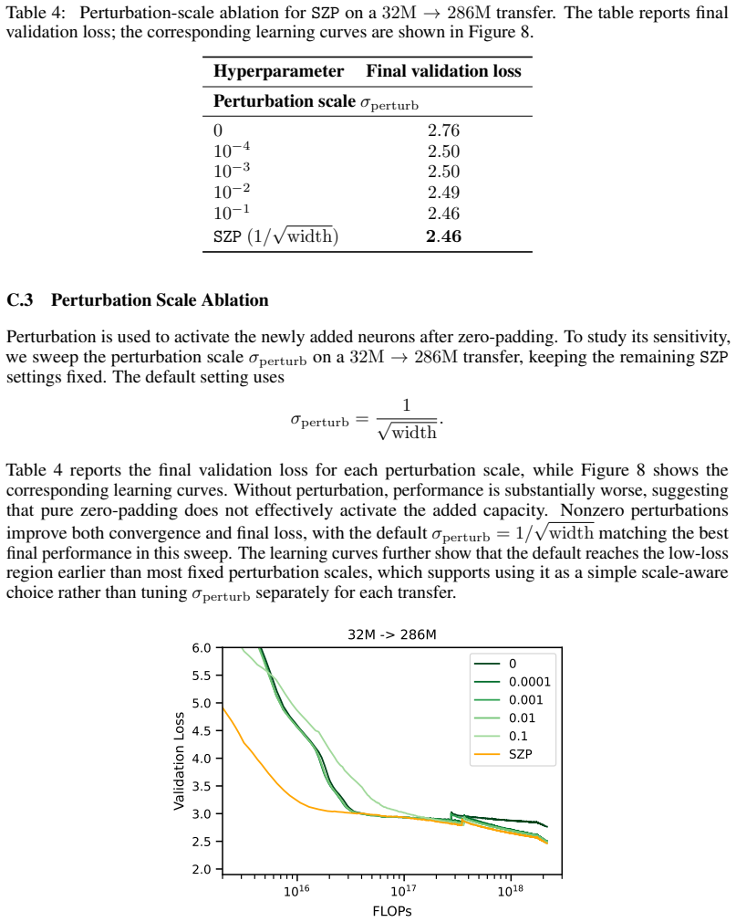
Hyperparameter Final validation loss Perturbation scaleσ perturb 0 2.76 10−4 2.50 10−3 2.50 10−2 2.49 10−1 2.46 SZP(1/ √ width)2.46 C.3 Perturbation Scale Ablation Perturbation is used to activate the newly added neurons after zero-padding. To study its sensitivity, we sweep the perturbation scale σperturb on a 32M→286M transfer, keeping the remaining SZP...
work page 2024
-
[33]
Parameter counts are rounded to the nearest million. dmodel nhead Head size Params (M) 128 2 64 14 256 4 64 32 512 8 64 77 768 12 64 134 1280 20 64 286 2048 32 64 610 3072 48 64 1200 For a simple mental illustration, a 1-head network with width 1 will have an attention tensor with 3 dimensions, one each forquery,key, andvalue, assuming no weight sharing. ...
work page 2048
-
[34]
Weight Decay.All experiments usezeroweight decay
for sub-billion parameter models. Weight Decay.All experiments usezeroweight decay. This isolates the effect of warmstarting from explicitℓ 2 regularization, avoiding confounding interactions between the two mechanisms. Warmup–Stable–Decay (WSD) Schedule.The learning rate follows a trapezoidal profile - letT be the total number of optimizer steps. For ηma...
work page 2024
-
[35]
D.3 Grid Search Results for Optimal Hyperparameters For the language-model experiments, we tune the peak learning rate ηmax and effective batch size at small base scales, then transfer the selected configuration to larger target scales using the µP 24 Table 6: Base-scale language-model hyperparameters selected forµP transfer. Params (M) Selectedη max Effe...
work page 1920
-
[36]
Together, the reported synthetic MLP experiments account for approximately10,143CPU-hours, or423CPU-days. For the reported language-model experiments, we report GPU-hour ranges based on the number of completed runs, hardware allocation, and typical wall-clock time per target scale. Including an allowance for debug and re-runs, this corresponds to roughly3...
work page 2023
-
[37]
For the subset overlapping with Hugging Face Open LLM Leaderboard v1, we follow the corresponding fixed few-shot settings: ARC-Challenge 25-shot, HellaSwag 10- shot, MMLU 5-shot, and WinoGrande 5-shot [Hugging Face, 2024a,b]. We additionally include OpenBookQA and PIQA as standard LIGHTEVALmultiple-choice tasks in the 0-shot setting. Across all six benchm...
work page 2016
-
[38]
Following Approach 3 of Hoffmann et al
For reference, we repeat the parametric form. Following Approach 3 of Hoffmann et al. [2022], we model the loss as a function of the number of parametersNand training tokensD: L(N, D) =E+ A N α + B Dβ , where E, A, α, B, β are fit to the data. The resulting fits capture the data well, with all R2 values exceeding0.99. Table 11: The fitted parameters and R...
work page 2022
discussion (0)
Sign in with ORCID, Apple, or X to comment. Anyone can read and Pith papers without signing in.