pith. sign in

arxiv: 2605.15284 · v1 · pith:HG6IZUGSnew · submitted 2026-05-14 · 💻 cs.LG

Tadpole: Autoencoders as Foundation Models for 3D PDEs with Online Learning

Pith reviewed 2026-05-19 16:36 UTC · model grok-4.3

classification 💻 cs.LG
keywords autoencodersfoundation models3D PDEsonline learningtransfer learningdynamics modelingparameter-efficient fine-tuninggenerative modeling
0
0 comments X

The pith

Autoencoders pre-trained on single-channel spatial crops of synthetic 3D PDE data transfer to dynamics learning and generation across diverse physical systems.

A machine-rendered reading of the paper's core claim, the machinery that carries it, and where it could break.

The paper introduces Tadpole as a foundation model for three-dimensional partial differential equations. It pre-trains an autoencoder solely on synthetic 3D PDE data generated online, using single-channel spatial crops to handle varying numbers of state variables and resolutions. This pre-training scales to the equivalent of hundreds of terabytes without storage overhead. The resulting representations support multiple downstream tasks, including accurate temporal dynamics modeling through a parameter-efficient fine-tuning approach that combines low-rank adaptation, latent-space transformations, and skip connections. A sympathetic reader would care because it points to a scalable way to reuse one base model across many different physical simulation problems instead of retraining from scratch for each system.

Core claim

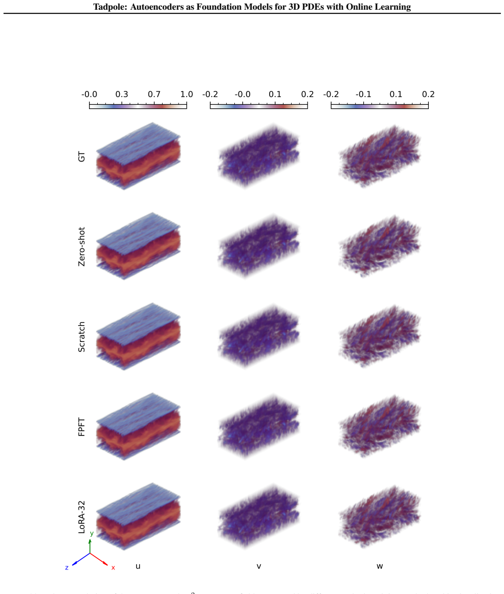
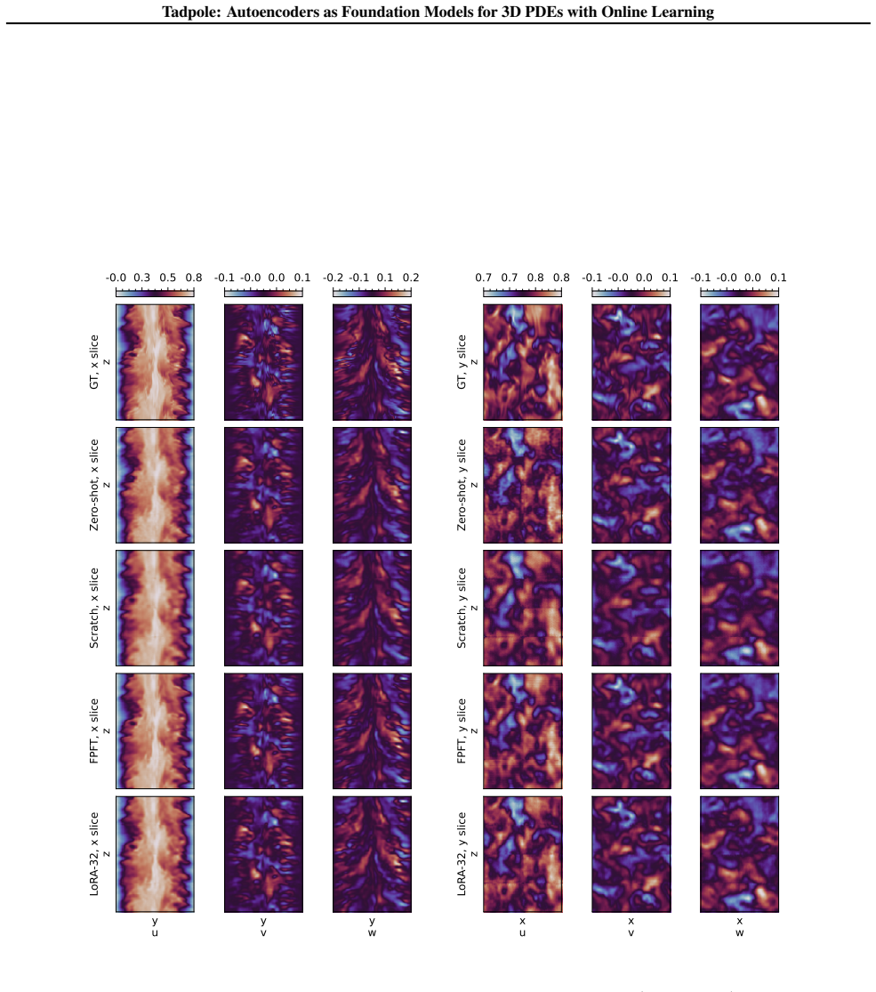
Tadpole is pre-trained as an autoencoder on single-channel spatial crops from an efficient online data-generation framework for 3D PDEs. This setup allows training on diverse synthetic data at massive scale. Although the pre-training task is reconstruction only, the learned representations transfer to heterogeneous physical systems. For dynamics learning, a novel fine-tuning strategy integrates low-rank adaptation, latent-space transformations, and reintroduced skip connections to achieve temporal modeling with a minimal number of trainable parameters. The model shows strong performance when applied to reconstruction, dynamics prediction, and generative modeling across different PDE systems.

What carries the argument

The central mechanism is the autoencoder pre-trained on single-channel spatial crops from online-generated 3D PDE data, paired with a parameter-efficient fine-tuning strategy that uses low-rank adaptation and latent-space transformations.

If this is right

  • One pre-trained model can handle multiple downstream tasks on 3D PDEs without full retraining.
  • Transfer across systems with different state variable counts and spatial resolutions becomes feasible.
  • Dynamics prediction requires only a small number of additional parameters after pre-training.
  • Online data generation removes storage limits and supports effectively unlimited training diversity.
  • Generative modeling of physical fields can reuse the same base representations.

Where Pith is reading between the lines

These are editorial extensions of the paper, not claims the author makes directly.

  • The same pre-training might reduce the need for domain-specific simulation code when adapting to new physics.
  • Extending the approach to real-world sensor data instead of purely synthetic inputs could test broader applicability.
  • Combining the latent representations with explicit boundary or initial condition inputs may further improve long-term prediction stability.

Load-bearing premise

Representations obtained by autoencoding single-channel spatial crops from synthetic 3D PDE data will transfer effectively to temporal dynamics modeling and generative tasks in different physical systems without large amounts of task-specific data or architecture changes.

What would settle it

Finding that fine-tuning Tadpole on a new physical system requires as many parameters or yields no better accuracy than training a fresh model from scratch on the target data would falsify the transfer claim.

Figures

Figures reproduced from arXiv: 2605.15284 by Benjamin Holzschuh, Felix Koehler, Nils Thuerey, Qiang Liu.

Figure 1
Figure 1. Figure 1: Overview of Tadpole: a) Tadpole is pre-trained as an autoencoder on single-channel crops of 3D PDE data generated on-the-fly by a GPU-based solver with an efficient buffer strategy to eliminate I/O and storage bottlenecks. b) The pre-trained Tadpole can be used for various downstream tasks, including autoencoding, dynamics learning with the novel Tadpole-DFT method, and generative modeling via latent flow … view at source ↗
Figure 2
Figure 2. Figure 2: Performance of Tadpole on the downstream autoencoding task (exact NRMSE values in [PITH_FULL_IMAGE:figures/full_fig_p006_2.png] view at source ↗
Figure 3
Figure 3. Figure 3: Visualizations of Tadpole-B zero-shot reconstruction on different datasets. Only velocity channels are shown here; additional ones are provided in Appendix A.7. The datasets feature high resolutions, ranging from 962 × 192 for TCF to 10243 for Iso. 5.2. Autoencoding Let D = C ×X ×Y ×Z denote the dimension of a 3D PDE state. To evaluate Tadpole’s autoencoding performance for unseen data, we consider four re… view at source ↗
Figure 4
Figure 4. Figure 4: Reconstruction NRMSE of Tadpole-B fine-tuned with different LoRA ranks on the Iso dataset. Increasing the rank approaches full-parameter fine-tuning. model pre-trained on a 500GB local dataset generated with the same PDEs and parameter distributions (cf [PITH_FULL_IMAGE:figures/full_fig_p006_4.png] view at source ↗
Figure 5
Figure 5. Figure 5: Performance of Tadpole on two distinct downstream dynamics tasks TBL and Iso. a) Prediction NRMSEES of different foundation models. Tadpole performs best on TBL, and second-best on Iso. b) The trainable parameters of different foundation models. Thanks to the LoRA introduced in the Tadpole-DFT method, only a very few parameters are fine-tuned in Tadpole, which makes it significantly smaller than the best-p… view at source ↗
Figure 6
Figure 6. Figure 6: Performance improvements on the dynamics test from pre-training of Tadpole. a) Relative NRMSEES of Tadpole-B fine￾tuned using various methods compared to the from-scratch variant. Increasing the LoRA rank in Tadpole-DFT consistently improves performance. b) Trainable parameters for different fine-tuning methods. The largest Tadpole-DFT variant utilizes only 22.3% of the trainable parameters required by the… view at source ↗
Figure 8
Figure 8. Figure 8: One-step NRMSEES of Tadpole-B fine-tuned with dif￾ferent Tadpole-DFT components. only achieves a lower final error but also converges faster and exhibits more stable training behavior than FPFT. LoRA Rank vs Capacity of S [PITH_FULL_IMAGE:figures/full_fig_p008_8.png] view at source ↗
Figure 9
Figure 9. Figure 9: Illustration of the distinction between learning the solution manifold and learning the induced dynamics. The curve represents a low-dimensional solution manifold M embedded in a higher-dimensional space. Tangent vectors along the manifold correspond to the intrinsic dynamics F(u) ∈ TuM, while the surrounding vector field illustrates the additional requirement of maintaining consistency with the manifold b… view at source ↗
Figure 10
Figure 10. Figure 10: Visualization of the reconstruction of TCF with crop-based and whole-domain inference for slices x = X/2 (left), and y = Y /2 (right). 17 [PITH_FULL_IMAGE:figures/full_fig_p017_10.png] view at source ↗
Figure 11
Figure 11. Figure 11: Visualization of the absolute error for the reconstruction of TCF with crop-based and whole-domain inference for slices x = X/2 (left), and y = Y /2 (right). 18 [PITH_FULL_IMAGE:figures/full_fig_p018_11.png] view at source ↗
Figure 12
Figure 12. Figure 12: shows the validation RMSE during FPFT and LoRA fine-tuning. FPFT fine-tuning exhibits many oscillations during training, especially at the start, whereas LoRA fine-tuning remains stable. This highlights LoRA fine-tuning’s ability to preserve pretrained knowledge, thereby avoiding training instabilities. 0 500 1000 1500 2000 2500 3000 3500 4000 Epochs 10 1 Validation RMSE LoRA 32 FPFT [PITH_FULL_IMAGE:fig… view at source ↗
Figure 13
Figure 13. Figure 13: One-step NRMSE of the Tadpole-B model with different sub-network sizes and LoRA ranks. Especially the latter positively affects performance. L o R A S k i p - C o n [PITH_FULL_IMAGE:figures/full_fig_p020_13.png] view at source ↗
Figure 14
Figure 14. Figure 14: One-step NRMSE of Tadpole-B fine-tuned with different Tadpole-DFT components. A.6. Detailed Metric Values of the Main Experiments In this section, we summarize the detailed metric values from the previous experiments [PITH_FULL_IMAGE:figures/full_fig_p020_14.png] view at source ↗
Figure 15
Figure 15. Figure 15: Volume rendering of the reconstructed 10243 Iso fields generated by different Tadpole training methods. 24 [PITH_FULL_IMAGE:figures/full_fig_p024_15.png] view at source ↗
Figure 16
Figure 16. Figure 16: Visualization of the reconstruction of Iso at the slice where x = X/2. GT, y slice z Zero-shot, y slice z Scratch, y slice z FPFT, y slice z x u LoRA-32, y slice z x v x w x p -2.5 -0.8 0.8 2.5 -2.7 -0.9 0.9 2.7 -2.8 -1.2 0.5 2.2 -4.1 -2.3 -0.5 1.2 [PITH_FULL_IMAGE:figures/full_fig_p025_16.png] view at source ↗
Figure 17
Figure 17. Figure 17: Visualization of the reconstruction of Iso at the slice where y = Y /2. 25 [PITH_FULL_IMAGE:figures/full_fig_p025_17.png] view at source ↗
Figure 18
Figure 18. Figure 18: Visualization of the reconstruction of Iso 1283 crops at the slice where x = X/2. GT, y slice z Zero-shot, y slice z Scratch, y slice z FPFT, y slice z x u LoRA-32, y slice z x v x w x p -0.8 -0.1 0.5 1.1 0.2 0.7 1.1 1.6 -1.0 -0.5 -0.0 0.4 -0.3 0.0 0.3 0.7 [PITH_FULL_IMAGE:figures/full_fig_p026_18.png] view at source ↗
Figure 19
Figure 19. Figure 19: Visualization of the reconstruction of Iso 1283 crops at the slice where y = Y /2. 26 [PITH_FULL_IMAGE:figures/full_fig_p026_19.png] view at source ↗
Figure 20
Figure 20. Figure 20: Visualization of the absolute error for the reconstruction of Iso 1283 crops at the slice where x = X/2. Zero-shot, y slice z Scratch, y slice z FPFT, y slice z x u LoRA-32, y slice z x v x w x p 0.0 0.1 0.2 0.3 0.0 0.1 0.2 0.3 0.0 0.1 0.2 0.2 0.0 0.1 0.2 0.4 [PITH_FULL_IMAGE:figures/full_fig_p027_20.png] view at source ↗
Figure 21
Figure 21. Figure 21: Visualization of the absolute error for the reconstruction of Iso 1283 crops at the slice where y = Y /2. 27 [PITH_FULL_IMAGE:figures/full_fig_p027_21.png] view at source ↗
Figure 22
Figure 22. Figure 22: Volume rendering of the reconstructed 962×192 TCF fields generated by different Tadpole training methods. This visualization confirms that all methods have successfully learned the large-scale structures of the data. Differences become apparent in the following visualizations of individual slices through the volume. 28 [PITH_FULL_IMAGE:figures/full_fig_p028_22.png] view at source ↗
Figure 23
Figure 23. Figure 23: Visualization of the reconstruction of TCF at the slice where x = X/2 and y = Y /2. 29 [PITH_FULL_IMAGE:figures/full_fig_p029_23.png] view at source ↗
Figure 24
Figure 24. Figure 24: Visualization of the absolute error for the reconstruction of TCF at the slice where x = X/2 and y = Y /2. 30 [PITH_FULL_IMAGE:figures/full_fig_p030_24.png] view at source ↗
Figure 25
Figure 25. Figure 25: Volume rendering of the reconstructed 5123 MHD fields generated by different Tadpole training methods. GT, x slice z Zero-shot, x slice z Scratch, x slice z FPFT, x slice z y u LoRA-32, x slice z y v y w y p y Bx y By y Bz y Ax y Ay y Az -0.7 -0.1 0.5 1.1 -1.0 -0.3 0.4 1.0 -0.7 -0.3 0.2 0.6 -0.6 -0.3 -0.0 0.3 -1.0 -0.3 0.5 1.2 -1.1 -0.4 0.2 0.9 -0.6 -0.3 0.1 0.5 -0.1 -0.0 0.1 0.2 -0.1 -0.0 0.0 0.1 -0.1 -0… view at source ↗
Figure 26
Figure 26. Figure 26: Visualization of the reconstruction of MHD at the slice where x = X/2. 31 [PITH_FULL_IMAGE:figures/full_fig_p031_26.png] view at source ↗
Figure 27
Figure 27. Figure 27: Visualization of the reconstruction of MHD at the slice where y = Y /2. GT, z slice y Zero-shot, z slice y Scratch, z slice y FPFT, z slice y x u LoRA-32, z slice y x v x w x p x Bx x By x Bz x Ax x Ay x Az -1.0 -0.3 0.4 1.1 -1.0 -0.3 0.4 1.0 -0.8 -0.4 0.0 0.4 -0.7 -0.4 -0.1 0.2 -1.0 -0.3 0.3 0.9 -1.2 -0.5 0.3 1.0 -0.6 -0.1 0.5 1.1 -0.1 -0.0 0.1 0.2 -0.1 -0.0 0.0 0.1 -0.1 -0.0 0.1 0.1 [PITH_FULL_IMAGE:fi… view at source ↗
Figure 28
Figure 28. Figure 28: Visualization of the reconstruction of MHD at the slice where z = Z/2. 32 [PITH_FULL_IMAGE:figures/full_fig_p032_28.png] view at source ↗
Figure 29
Figure 29. Figure 29: Visualization of the reconstruction of MHD 1283 crops at the slice where y = Y /2. GT, z slice y Zero-shot, z slice y Scratch, z slice y FPFT, z slice y x u LoRA-32, z slice y x v x w x p x Bx x By x Bz x Ax x Ay x Az -0.5 -0.2 0.1 0.5 -0.3 -0.1 0.1 0.4 -0.6 -0.3 -0.0 0.3 -0.7 -0.5 -0.2 0.1 -0.8 -0.3 0.3 0.9 -0.5 -0.1 0.3 0.8 -0.5 0.1 0.7 1.3 -0.0 0.0 0.1 0.1 -0.1 -0.0 0.0 0.1 0.0 0.1 0.1 0.2 [PITH_FULL_… view at source ↗
Figure 30
Figure 30. Figure 30: Visualization of the reconstruction of MHD 1283 crops at the slice where z = Z/2. 33 [PITH_FULL_IMAGE:figures/full_fig_p033_30.png] view at source ↗
Figure 31
Figure 31. Figure 31: Visualization of the absolute error for the reconstruction of MHD 1283 crops at the slice where y = Y /2. Zero-shot, z slice y Scratch, z slice y FPFT, z slice y x u LoRA-32, z slice y x v x w x p x Bx x By x Bz x Ax x Ay x Az 0.0 0.1 0.1 0.2 0.0 0.0 0.1 0.1 0.0 0.1 0.1 0.2 0.0 0.1 0.1 0.2 0.0 0.1 0.2 0.3 0.0 0.1 0.1 0.2 0.0 0.1 0.2 0.3 0.0 0.0 0.0 0.0 0.0 0.0 0.0 0.0 0.0 0.0 0.0 0.0 [PITH_FULL_IMAGE:fig… view at source ↗
Figure 32
Figure 32. Figure 32: Visualization of the absolute error for the reconstruction of MHD 1283 crops at the slice where z = Z/2. 34 [PITH_FULL_IMAGE:figures/full_fig_p034_32.png] view at source ↗
Figure 33
Figure 33. Figure 33: Volume rendering of the reconstructed 2243 TBL fields generated by different Tadpole training methods. 35 [PITH_FULL_IMAGE:figures/full_fig_p035_33.png] view at source ↗
Figure 34
Figure 34. Figure 34: Visualization of the reconstruction of TBL at the slice where x = X/2. GT, y slice z Zero-shot, y slice z Scratch, y slice z FPFT, y slice z x u LoRA-32, y slice z x v x w x p 0.5 0.6 0.8 1.0 -0.2 -0.1 0.1 0.2 -0.2 -0.0 0.1 0.2 -0.0 0.0 0.0 0.0 [PITH_FULL_IMAGE:figures/full_fig_p036_34.png] view at source ↗
Figure 35
Figure 35. Figure 35: Visualization of the reconstruction of TBL at the slice where y = Y /2. 36 [PITH_FULL_IMAGE:figures/full_fig_p036_35.png] view at source ↗
Figure 36
Figure 36. Figure 36: Visualization of absolute error for the reconstruction of TBL at the slice where x = X/2. Zero-shot, y slice z Scratch, y slice z FPFT, y slice z x u LoRA-32, y slice z x v x w x p 0.0 0.0 0.0 0.1 0.0 0.0 0.0 0.1 0.0 0.0 0.0 0.1 0.0 0.0 0.0 0.0 [PITH_FULL_IMAGE:figures/full_fig_p037_36.png] view at source ↗
Figure 37
Figure 37. Figure 37: Visualization of absolute error for the reconstruction of TBL at the slice where y = Y /2. 37 [PITH_FULL_IMAGE:figures/full_fig_p037_37.png] view at source ↗
Figure 38
Figure 38. Figure 38: Visualization of the prediction (left) of Iso and the corresponding absolute error (right) at the first rollout step and the slice where z = Z/2. 38 [PITH_FULL_IMAGE:figures/full_fig_p038_38.png] view at source ↗
Figure 39
Figure 39. Figure 39: Visualization of the prediction (left) of Iso and the corresponding absolute error (right) at the second rollout step and the slice where z = Z/2. Ground Truth, z slice y Walrus, z slice y DPOT-S, z slice y MORPH-S, z slice y x u Tadpole-Lora32, z slice y x v x w x p -0.6 -0.1 0.5 1.1 -0.5 0.1 0.7 1.4 -1.2 -0.3 0.5 1.4 -0.2 0.0 0.3 0.6 Walrus, z slice y DPOT-S, z slice y MORPH-S, z slice y x u Tadpole-Lor… view at source ↗
Figure 40
Figure 40. Figure 40: Visualization of the prediction (left) of Iso and the corresponding absolute error (right) at the third rollout step and the slice where z = Z/2. 39 [PITH_FULL_IMAGE:figures/full_fig_p039_40.png] view at source ↗
Figure 41
Figure 41. Figure 41: Visualization of the prediction (left) of TBL and the corresponding absolute error (right) at the first rollout step and the slice where z = Z/2. Ground Truth, z slice y Walrus, z slice y DPOT-S, z slice y MORPH-S, z slice y x u Tadpole-Lora32, z slice y x v x w 0.3 0.6 0.8 1.0 -0.1 -0.0 0.1 0.1 -0.2 -0.1 0.0 0.1 Walrus, z slice y DPOT-S, z slice y MORPH-S, z slice y x u Tadpole-Lora32, z slice y x v x w … view at source ↗
Figure 42
Figure 42. Figure 42: Visualization of the prediction (left) of TBL and the corresponding absolute error (right) at the second rollout step and the slice where z = Z/2. 40 [PITH_FULL_IMAGE:figures/full_fig_p040_42.png] view at source ↗
Figure 43
Figure 43. Figure 43: Visualization of the prediction (left) of TBL and the corresponding absolute error (right) at the third rollout step and the slice where z = Z/2. B. Dataset and Online Learning Setups B.1. Pre-training Dataset A significant challenge in training 3D physics foundation models is the production, storage, and efficient loading of large-scale spatiotemporal datasets. To illustrate the magnitude of this bottlen… view at source ↗
Figure 44
Figure 44. Figure 44: Radially shell-aggregated magnitude spectra (100 samples per distribution). Row 1 (GN & TFS): Gaussian (white) noise (GN) exhibits quadratic growth due to the volume of spherical shells in 3D Fourier space. The Truncated Fourier Series (TFS) initializers show distinct spectral cutoffs determined by klimit. Note that TFS-D exhibits vertical variation due to its randomized normalization bounds. Row 2 (DN & … view at source ↗
Figure 45
Figure 45. Figure 45: This collection of all shell-aggregated spectra across 100,000 samples (about one tenth of the pre-training amount) from the simulation server highlights the diversity of states exposed to the foundational pre-training of Tadpole. but also further diffuse them. The Burgers equation develops noticeable shocks, as evidenced by a richer spectral content than in the initialization. Also, the pattern-forming K… view at source ↗
Figure 46
Figure 46. Figure 46: Distribution of Fourier coefficient magnitude across radially aggregated bins for a spectral analysis of the 643 training crops based on 100,000 samples from the simulation server (about 10% of the amount of data used for Tadpole B-size pre-taining). Each row represents a different PDE (according to [PITH_FULL_IMAGE:figures/full_fig_p048_46.png] view at source ↗
Figure 47
Figure 47. Figure 47: Network architecture of Tadpole based on P3D (Holzschuh et al., 2026). 54 [PITH_FULL_IMAGE:figures/full_fig_p054_47.png] view at source ↗
Figure 48
Figure 48. Figure 48: Network architecture of S based. C.2. Training Objective The loss function for the VAE consists of three terms: a reconstruction loss, a KL-divergence regularization term, and an adversarial loss term weighted by λA. The discriminator loss function encourages correct classification of real and reconstructed samples. For the adversarial loss, the discriminator A outputs a scalar score A(ut) indicating the … view at source ↗
read the original abstract

We introduce Tadpole, a novel foundation model for three-dimensional partial differential equations (PDEs) that addresses key challenges in transferability, scalability to high dimensionality, and multi-functionality. Tadpole is pre-trained as an autoencoder on synthetic 3D PDE data generated by an efficient online data-generation framework. This enables large-scale, diverse training without storage or I/O overhead, demonstrated by scaling to an equivalent of hundreds of terabytes of training data. By autoencoding single-channel spatial crops, Tadpole learns rich and transferable representations across heterogeneous physical systems with varying numbers of state variables and spatial resolutions. Although pre-trained solely as an autoencoder, Tadpole can be efficiently applied for multiple downstream tasks beyond reconstruction, including dynamics learning and generative modeling. For dynamics learning, we propose a novel parameter-efficient fine-tuning strategy that integrates low-rank adaptation, latent-space transformations, and reintroduced skip connections, achieving accurate temporal modeling with a minimal number of trainable parameters. Tadpole demonstrates strong fine-tuning performance across various downstream tasks, highlighting its versatility and effectiveness as a foundation model for 3D PDE learning. Source code and pre-trained weights of Tadpole are available at https://github.com/tum-pbs/tadpole

Editorial analysis

A structured set of objections, weighed in public.

Desk editor's note, referee report, simulated authors' rebuttal, and a circularity audit. Tearing a paper down is the easy half of reading it; the pith above is the substance, this is the friction.

Referee Report

2 major / 2 minor

Summary. The manuscript introduces Tadpole, a foundation model for 3D PDEs pre-trained as an autoencoder on synthetic data generated via an online framework that scales to hundreds of terabytes without storage overhead. Pre-training uses single-channel spatial crops to learn representations claimed to transfer across heterogeneous physical systems with varying numbers of state variables and resolutions. A parameter-efficient fine-tuning strategy combining low-rank adaptation, latent-space transformations, and reintroduced skip connections is proposed for downstream tasks including dynamics learning and generative modeling, with the authors reporting strong fine-tuning performance. Source code and pre-trained weights are released.

Significance. If the transferability and efficiency claims hold under rigorous validation, Tadpole would offer a meaningful step toward foundation models for scientific machine learning on high-dimensional 3D PDEs, where data scale and task diversity are persistent bottlenecks. The online data-generation approach and the explicit parameter-efficient fine-tuning recipe are practical contributions. The public release of code and weights is a clear strength that supports reproducibility and community follow-up.

major comments (2)
  1. [Abstract and pre-training section] Abstract and the description of the pre-training objective: the central claim that an autoencoder trained only on reconstruction of single-channel static spatial crops produces latents sufficient for accurate temporal dynamics modeling on multi-state systems rests on the fine-tuning strategy compensating for the complete absence of temporal derivatives and cross-channel interactions in pre-training; this assumption is load-bearing and requires explicit ablation evidence (e.g., comparison of latent features with and without temporal context) to substantiate transfer across differing numbers of state variables.
  2. [Fine-tuning and dynamics learning section] Fine-tuning strategy description: the integration of LoRA, latent transformations, and skip connections is presented as achieving accurate time-stepping with minimal trainable parameters, yet the manuscript does not quantify how much of the dynamical information is recovered by each component versus what must be learned from scratch; without such decomposition, the efficiency claim cannot be fully evaluated.
minor comments (2)
  1. [Method] Notation for the latent-space transformations should be defined more explicitly, including the precise form of the skip-connection reintroduction.
  2. [Results] Figure captions and axis labels in the results visualizations would benefit from clearer indication of which PDE system and resolution each panel corresponds to.

Simulated Author's Rebuttal

2 responses · 0 unresolved

We thank the referee for their constructive feedback and recommendation for major revision. We address each major comment below with clarifications and commitments to strengthen the manuscript through additional analyses.

read point-by-point responses
  1. Referee: [Abstract and pre-training section] Abstract and the description of the pre-training objective: the central claim that an autoencoder trained only on reconstruction of single-channel static spatial crops produces latents sufficient for accurate temporal dynamics modeling on multi-state systems rests on the fine-tuning strategy compensating for the complete absence of temporal derivatives and cross-channel interactions in pre-training; this assumption is load-bearing and requires explicit ablation evidence (e.g., comparison of latent features with and without temporal context) to substantiate transfer across differing numbers of state variables.

    Authors: We appreciate the referee highlighting this key assumption. The pre-training on single-channel static crops is intentionally designed to learn general spatial representations that can transfer across heterogeneous PDE systems. The manuscript shows this transfer empirically via strong fine-tuning performance on dynamics tasks with varying state variables and resolutions. To directly address the request for explicit ablation evidence, we will add in the revised manuscript comparisons of latent features and downstream performance with versus without temporal context during fine-tuning, as well as ablations isolating cross-channel effects. These will substantiate the transferability claims. revision: yes

  2. Referee: [Fine-tuning and dynamics learning section] Fine-tuning strategy description: the integration of LoRA, latent transformations, and skip connections is presented as achieving accurate time-stepping with minimal trainable parameters, yet the manuscript does not quantify how much of the dynamical information is recovered by each component versus what must be learned from scratch; without such decomposition, the efficiency claim cannot be fully evaluated.

    Authors: We agree that a quantitative breakdown of each fine-tuning component's contribution would strengthen the efficiency evaluation. The current results demonstrate overall low parameter counts and accurate time-stepping, but to provide the requested decomposition, we will include in the revised manuscript ablation studies that enable or disable LoRA, latent-space transformations, and skip connections individually. These will report trainable parameter counts and prediction errors for each variant, clarifying the dynamical information recovered by each versus what is learned from scratch. revision: yes

Circularity Check

0 steps flagged

No circularity: empirical results from distinct pre-training and fine-tuning objectives

full rationale

The paper is an empirical ML study introducing Tadpole as a pre-trained autoencoder on synthetic 3D PDE spatial crops, followed by parameter-efficient fine-tuning for dynamics and generative tasks. No derivation chain exists that reduces predictions or claims to inputs by construction; performance claims rest on observed transfer across systems rather than any fitted parameter being renamed as a prediction or any self-citation defining the outcome. The pre-training objective (reconstruction of single-channel crops) and downstream objectives (temporal modeling via LoRA and skip connections) are explicitly separated, with results validated through experiments on heterogeneous PDEs. This is self-contained against external benchmarks of model performance.

Axiom & Free-Parameter Ledger

1 free parameters · 1 axioms · 1 invented entities

The central claim depends on the assumption that autoencoder pre-training on synthetic spatial crops produces representations that generalize to dynamics and generation tasks, plus standard deep-learning assumptions about optimization and representation power.

free parameters (1)
  • LoRA rank and scaling factors
    Hyperparameters controlling the low-rank adaptation matrices in the fine-tuning stage; their values are chosen to achieve the reported performance.
axioms (1)
  • domain assumption Autoencoding single-channel spatial crops yields representations transferable across PDEs with different numbers of state variables and resolutions
    Invoked when claiming cross-system transferability from the pre-training procedure described in the abstract.
invented entities (1)
  • Tadpole model no independent evidence
    purpose: Foundation model for 3D PDEs
    Newly introduced architecture and training framework presented in the paper.

pith-pipeline@v0.9.0 · 5756 in / 1432 out tokens · 57350 ms · 2026-05-19T16:36:58.524944+00:00 · methodology

discussion (0)

Sign in with ORCID, Apple, or X to comment. Anyone can read and Pith papers without signing in.

Lean theorems connected to this paper

Citations machine-checked in the Pith Canon. Every link opens the source theorem in the public Lean library.

What do these tags mean?
matches
The paper's claim is directly supported by a theorem in the formal canon.
supports
The theorem supports part of the paper's argument, but the paper may add assumptions or extra steps.
extends
The paper goes beyond the formal theorem; the theorem is a base layer rather than the whole result.
uses
The paper appears to rely on the theorem as machinery.
contradicts
The paper's claim conflicts with a theorem or certificate in the canon.
unclear
Pith found a possible connection, but the passage is too broad, indirect, or ambiguous to say the theorem truly supports the claim.

Reference graph

Works this paper leans on

14 extracted references · 14 canonical work pages · 1 internal anchor

  1. [1]

    URL https://proceedings.mlr.press/ v235/chen24n.html. Cox, S. and Matthews, P. Exponential Time Dif- ferencing for Stiff Systems. Journal of Compu- tational Physics , 176(2):430–455, 2002. ISSN 0021-9991. doi: https://doi.org/10.1006/jcph.2002

  2. [2]

    URL https://www.sciencedirect.com/ science/article/pii/S0021999102969950. Ding, N., Qin, Y ., Yang, G., Wei, F., Yang, Z., Su, Y ., Hu, S., Chen, Y ., Chan, C.-M., Chen, W., Yi, J., Zhao, W., Wang, X., Liu, Z., Zheng, H.-T., Chen, J., Liu, Y ., Tang, J., Li, J., and Sun, M. Parameter-efficient fine-tuning of large-scale pre-trained language models. Nature...

  3. [3]

    doi: https://doi.org/10.1016/j.neucom.2021.04

  4. [4]

    Holzschuh, B., Liu, Q., Kohl, G., and Thuerey, N

    URL https://www.sciencedirect.com/ science/article/pii/S0925231221006706. Holzschuh, B., Liu, Q., Kohl, G., and Thuerey, N. PDE- transformer: Efficient and versatile transformers for physics simulations. In Singh, A., Fazel, M., Hsu, D., Lacoste-Julien, S., Berkenkamp, F., Maharaj, T., Wagstaff, K., and Zhu, J. (eds.), International Confer- ence on Machin...

  5. [5]

    URL https:// epubs.siam.org/doi/10.1137/24M1636071

    doi: 10.1137/24M1636071. URL https:// epubs.siam.org/doi/10.1137/24M1636071. Jollie, D., Sun, J., Zhang, Z., and Schaeffer, H. Time- Series Forecasting, Knowledge Distillation, and Refine- ment within a Multimodal PDE Foundation Model, 2024. URL https://arxiv.org/abs/2409.11609. Kassam, A.-K. and Trefethen, L. N. Fourth-Order Time- Stepping for Stiff PDEs...

  6. [6]

    Geometric GAN

    URL https://openreview.net/forum? id=n7qGCmluZr. Li, Y ., Perlman, E., Wan, M., Yang, Y ., Meneveau, C., Burns, R., Chen, S., Szalay, A., and Eyink, G. A public turbulence database cluster and applications to study Lagrangian evolution of velocity increments in turbulence. Journal of Turbulence, 9:N31, 2008. doi: 10.1080/14685240802376389. URL https://doi...

  7. [7]

    Siddik, A

    URL https://openreview.net/forum? id=0r9mhjRv1E. Siddik, A. B., Oyen, D., Most, A., Kucer, M., and Biswas, A. SPUS: A Lightweight and Parameter-Efficient Foun- dation Model for PDEs, 2025. URL https://arxiv. org/abs/2510.01370. Song, Z., Yuan, J., and Yang, H. FMint: Bridging Human Designed and Data Pretrained Models for Differential Equation Foundation M...

  8. [8]

    transport crop

    URL https://openreview.net/forum? id=GLDMCwdhTK. Ye, Z., Liu, Z., Wu, B., Jiang, H., Chen, L., Zhang, M., Huang, X., Meng, Q., Zou, J., Liu, H., and Dong, B. PDEformer-2: A Versatile Foundation Model for Two- Dimensional Partial Differential Equations, 2025. URL https://arxiv.org/abs/2507.15409. Zhang, D., Feng, T., Xue, L., Wang, Y ., Dong, Y ., and Tang...

  9. [9]

    If this buffer fills up, the simulator pauses, preventing memory overflows

    Transmission Queue (FIFO): The simulation server pushes completed transport samples into a finite-sized First-In- First-Out buffer. If this buffer fills up, the simulator pauses, preventing memory overflows. From this queue, data is sent to all participating training GPUs in a round-robin fashion

  10. [10]

    New frames are received here before being processed for the training cache

    Local Staging Buffer (FIFO): Each training GPU maintains an incoming “mailbox” queue. New frames are received here before being processed for the training cache

  11. [11]

    Background threads continuously replenish this cache

    Consumer Cache (MFU): On the training side, frames are moved from the staging buffer into a larger local cache governed by a Most-Frequently-Used (MFU) replacement policy. Background threads continuously replenish this cache. The training loop samples batches from the Consumer Cache rather than the stream directly. This decouples the training step time fr...

  12. [12]

    The corrupted trajectory is immediately discarded

  13. [13]

    The specific simulator instance responsible is reset with a new random seed and parameters

  14. [14]

    If the error counter exceeds a tolerance threshold (set to 10 events per training run), the entire training process is halted to allow for debugging

    A global error counter is incremented. If the error counter exceeds a tolerance threshold (set to 10 events per training run), the entire training process is halted to allow for debugging. This ensures that the model is never exposed to corrupted gradients. Multi-Node and Distributed Training Our default configuration utilizes a single node with four GPUs...