The Lumina Project: The Demographics of Active Galactic Nuclei from Quasars to Little Red Dots at zgeq 3
Pith reviewed 2026-06-30 15:10 UTC · model grok-4.3
The pith
An empirical model from a large cosmological simulation reproduces AGN luminosity functions for both quasars and Little Red Dots at z ≥ 3.
A machine-rendered reading of the paper's core claim, the machinery that carries it, and where it could break.
Core claim
The central claim is that SMBHs with masses up to 10^7 solar masses remain in the LRD phase with a 30 percent duty cycle, and that applying standard bolometric and extinction corrections plus 0.3 dex log-normal scatter in bolometric luminosity allows the simulated population to reproduce the observed AGN luminosity functions and clustering from quasars down to Little Red Dots at z ≥ 3, while the same population drives the modeled He II reionization.
What carries the argument
The empirical AGN model that assigns SMBHs below 10^7 solar masses to an LRD phase with 30 percent duty cycle and applies luminosity corrections plus scatter to map simulated black holes onto multi-band observations.
If this is right
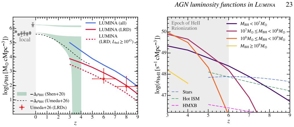
- The modeled AGN population is the dominant driver of He II reionization in the simulation.
- Number densities of AGN and LRDs evolve with redshift in a way that can be directly compared to future surveys.
- The integrated black hole mass density receives a calculable contribution from the LRD phase at high redshift.
- The same framework supports building general population-synthesis models of high-redshift AGN that include LRDs.
Where Pith is reading between the lines
- The model implies that Little Red Dots mark a distinct early growth stage for black holes that later transition into quasars.
- Varying the duty cycle with redshift or mass could alter the timing of helium reionization in testable ways.
- The required luminosity scatter suggests that future multi-epoch observations might detect variability differences between LRDs and quasars.
- Extending the model to include feedback effects on host galaxies could link AGN demographics to galaxy quenching at these epochs.
Load-bearing premise
Supermassive black holes with masses up to 10 million solar masses remain in the Little Red Dot phase with a fixed 30 percent duty cycle.
What would settle it
An observation that the spatial clustering amplitude of Little Red Dots at z ≥ 3 deviates significantly from the prediction based on the underlying galaxy distribution in the simulation, or that the bright-end quasar luminosity function cannot be recovered with 0.3 dex scatter.
Figures
read the original abstract
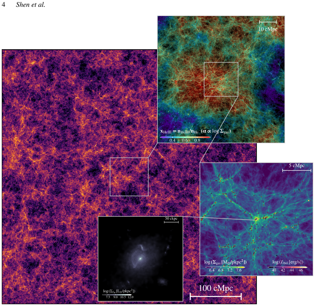
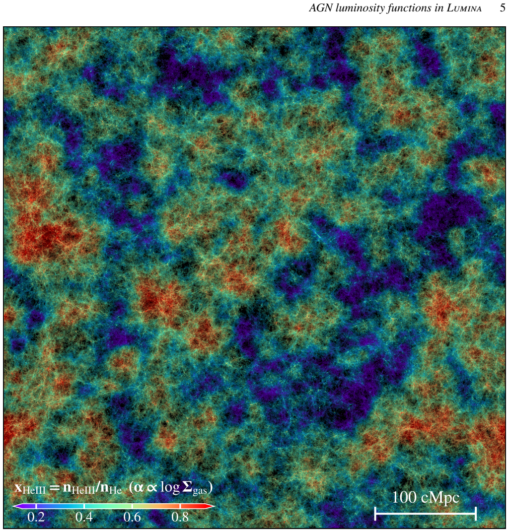
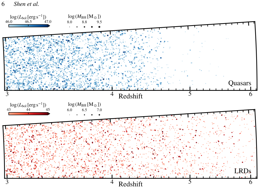
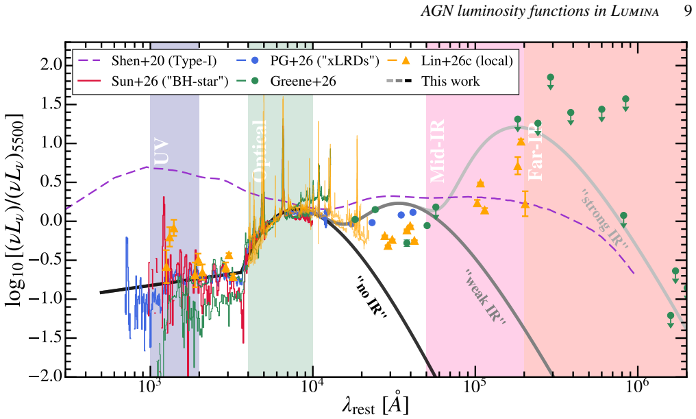
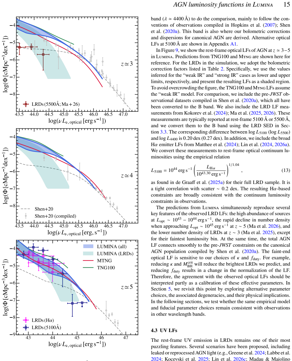
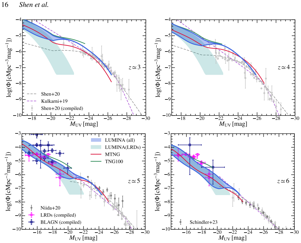
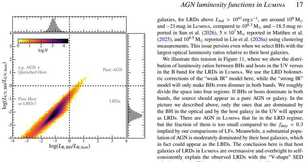
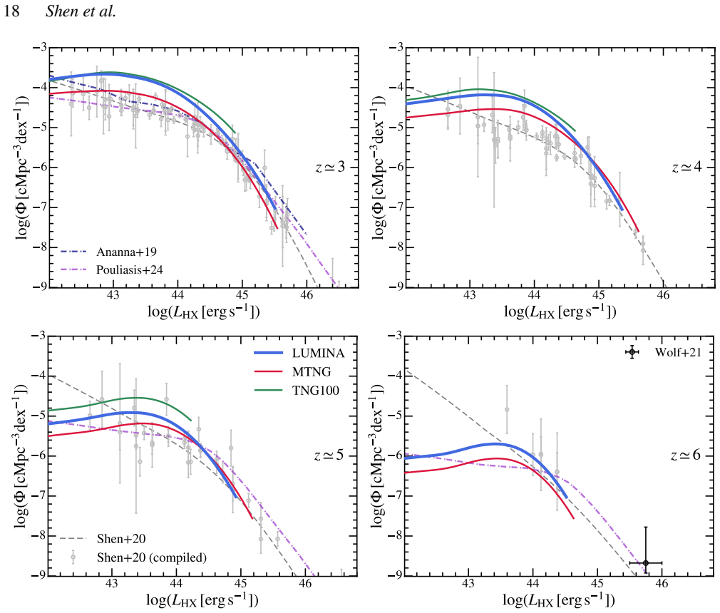
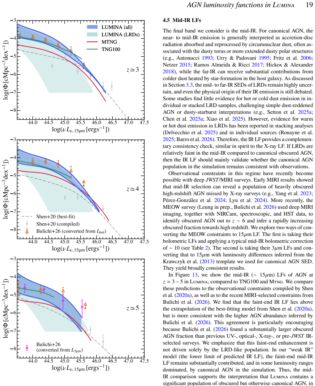
High-redshift active galactic nuclei (AGN) serve as powerful probes of early black-hole growth, galaxy formation, and the evolving intergalactic medium (IGM). In this work, we use Lumina, a cosmological radiation-hydrodynamic simulation spanning the epochs of hydrogen and helium reionization, which combines a large $(500\,{\rm cMpc})^3$ volume with $2\times 6000^3$ resolution elements, to explore high-redshift AGN. The simulation self-consistently follows hundreds of millions of galaxies and supermassive black holes (SMBHs), together with their impact on the ionization and thermal state of the IGM. We exploit this uniquely large dynamic range to predict multi-band AGN luminosity functions (LFs) at $z \geq 3$, from hard X-rays to the mid-infrared. These predictions encompass both moderately luminous quasars and the faint ``Little Red Dots'' (LRDs) uncovered by JWST. We develop an empirical model that maps simulated SMBHs onto observed AGN using bolometric and extinction/absorption corrections for canonical AGN and LRDs, and in which SMBHs with $M_{\rm BH}\leq 10\,M_{\rm seed} \sim 10^{7}\,{\rm M}_{\odot}$ stay in the LRD phase with a duty cycle of $30\%$. This simple framework reproduces the observed LFs and clustering of LRDs. Meanwhile, the pre-JWST quasar LF constraints are recovered, although we find that a $\sim 0.3$ dex log-normal scatter in bolometric luminosity is required to reproduce the bright end. We place the simulated AGN population in the cosmological context by quantifying the redshift evolution of AGN and LRD number densities, and their contributions to the integrated BH mass densities. The same AGN population is the dominant driver for the HeII reionization modelled self-consistently in Lumina. This empirical AGN model paves the way for general population-synthesis models of high-redshift AGN, including LRDs, in a unified cosmological framework.
Editorial analysis
A structured set of objections, weighed in public.
Referee Report
Summary. The paper presents results from the Lumina cosmological radiation-hydrodynamic simulation (500 cMpc volume, 2×6000³ resolution) to predict multi-band AGN luminosity functions at z≥3, encompassing both quasars and JWST-discovered Little Red Dots (LRDs). An empirical model maps simulated SMBHs to observed AGN via bolometric/extinction corrections, with SMBHs below ~10^7 M_⊙ assigned a 30% duty cycle in the LRD phase; a ~0.3 dex log-normal scatter in bolometric luminosity is introduced to match the bright end. The framework is stated to reproduce observed LFs and LRD clustering, recover pre-JWST quasar constraints, quantify AGN number densities and BH mass density contributions, and identify the simulated AGN as the dominant driver of self-consistently modeled HeII reionization.
Significance. If the empirical mapping can be shown to have predictive power beyond parameter tuning, the work supplies a unified cosmological framework linking high-z quasars and LRDs within a single large-volume simulation that self-consistently treats reionization. The large dynamic range and explicit connection to IGM thermal/ionization state are clear strengths for population-synthesis modeling.
major comments (3)
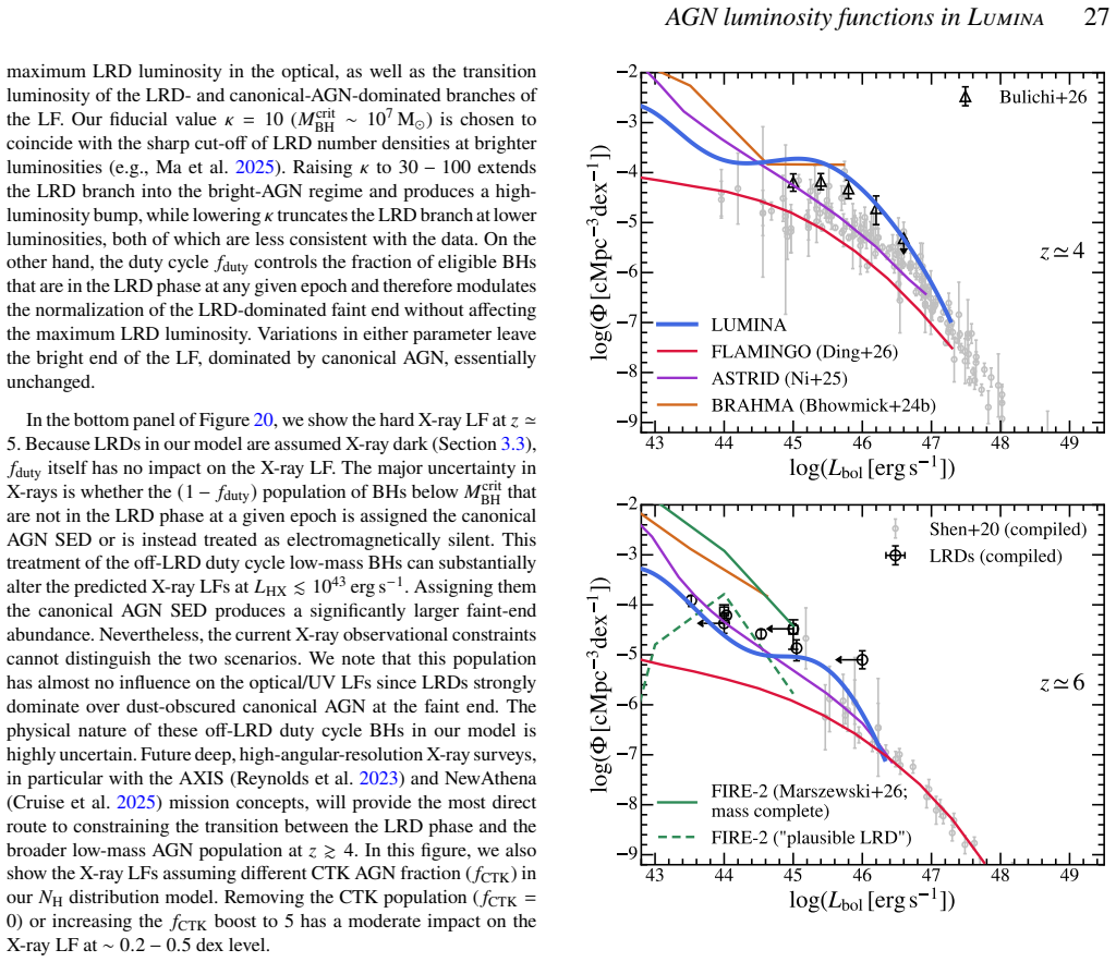
- [Abstract / empirical model] Abstract and empirical model description: the 30% duty cycle for SMBHs with M_BH ≤ 10 M_seed ~10^7 M_⊙ is stated to be chosen so that the model reproduces the JWST LRD luminosity function. Because the central claim is that the framework 'reproduces the observed LFs', this choice renders the match partly by construction; an independent validation (e.g., using the duty cycle fixed from other observables and then predicting the LF) is required for the reproduction to be non-circular.
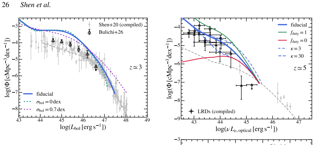
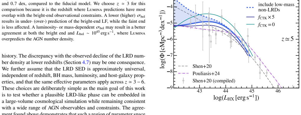
- [Abstract] Abstract: the statement that '~0.3 dex log-normal scatter in bolometric luminosity is required to reproduce the bright end' is load-bearing for the quasar LF recovery claim, yet no quantitative comparison (with vs. without scatter) or goodness-of-fit metric is referenced. This needs to be shown explicitly, for example via a table or figure comparing model LFs at the bright end.
- [Abstract] Abstract: the claim that clustering of LRDs is reproduced must be shown to be independent of the duty-cycle tuning. If the duty cycle only rescales number density without altering the spatial bias of the selected objects, this should be demonstrated; otherwise any additional parameter adjustment for clustering statistics must be reported.
minor comments (1)
- Notation for M_seed and the precise definition of the LRD phase should be clarified in the main text to avoid ambiguity with the abstract's 'M_BH ≤ 10 M_seed ~10^7 M_⊙'.
Simulated Author's Rebuttal
We thank the referee for their careful reading and valuable comments on our manuscript. We address each of the major comments below and indicate the revisions we will make.
read point-by-point responses
-
Referee: [Abstract / empirical model] Abstract and empirical model description: the 30% duty cycle for SMBHs with M_BH ≤ 10 M_seed ~10^7 M_⊙ is stated to be chosen so that the model reproduces the JWST LRD luminosity function. Because the central claim is that the framework 'reproduces the observed LFs', this choice renders the match partly by construction; an independent validation (e.g., using the duty cycle fixed from other observables and then predicting the LF) is required for the reproduction to be non-circular.
Authors: We agree that the 30% duty cycle parameter was chosen specifically to reproduce the observed JWST LRD luminosity function, as explicitly stated in the abstract and methods. This does make the match to the LRD LF partly by construction. The framework's strength lies in its ability to simultaneously match multiple observables, including the quasar LF, clustering, and reionization history, within a single self-consistent simulation. For the revision, we will add a new subsection discussing independent motivations for the duty cycle value (e.g., from AGN variability studies at lower redshifts) and present results for a range of duty cycle values to show robustness. revision: yes
-
Referee: [Abstract] Abstract: the statement that '~0.3 dex log-normal scatter in bolometric luminosity is required to reproduce the bright end' is load-bearing for the quasar LF recovery claim, yet no quantitative comparison (with vs. without scatter) or goodness-of-fit metric is referenced. This needs to be shown explicitly, for example via a table or figure comparing model LFs at the bright end.
Authors: We acknowledge that the manuscript does not include an explicit quantitative comparison of the luminosity function with and without the scatter. In the revised manuscript, we will add a figure showing the bright-end quasar LF both with and without the 0.3 dex log-normal scatter, along with a table of goodness-of-fit metrics (e.g., reduced chi-squared) to the observational data points. revision: yes
-
Referee: [Abstract] Abstract: the claim that clustering of LRDs is reproduced must be shown to be independent of the duty-cycle tuning. If the duty cycle only rescales number density without altering the spatial bias of the selected objects, this should be demonstrated; otherwise any additional parameter adjustment for clustering statistics must be reported.
Authors: The duty cycle is a uniform rescaling factor applied to the number of active SMBHs and does not alter the spatial distribution or halo bias of the underlying population, which is set by the simulation. We will demonstrate this explicitly in the revised version by computing the two-point correlation function for the LRD population at different duty cycle values (e.g., 10%, 30%, 50%) and showing that the bias factor remains consistent within uncertainties. revision: yes
Circularity Check
30% LRD duty cycle and 0.3 dex scatter are parameters tuned to reproduce observed LFs
specific steps
-
fitted input called prediction
[Abstract]
"SMBHs with M_BH≤10 M_seed ∼10^7 M_⊙ stay in the LRD phase with a duty cycle of 30%. This simple framework reproduces the observed LFs and clustering of LRDs. ... although we find that a ∼0.3 dex log-normal scatter in bolometric luminosity is required to reproduce the bright end."
The duty cycle fraction and scatter amplitude are stated as chosen/adjusted specifically so the model matches the observed luminosity functions; the subsequent claim that the framework 'reproduces' those LFs therefore reduces to the input choice by construction.
full rationale
The central claim that the empirical model reproduces observed LFs and clustering rests on an explicitly fitted duty cycle (set to 30% for M_BH ≤ 10^7 M_⊙) and luminosity scatter (0.3 dex) chosen so the simulated population matches the JWST LRD LF and bright-end quasar LF. This makes the LF reproduction a fitted outcome rather than an a-priori prediction from the underlying simulation. Clustering reproduction is not shown to require additional tuning and may retain some independence, but the load-bearing LF match is by construction. No other circular steps (self-citation chains or ansatz smuggling) are evident from the provided text.
Axiom & Free-Parameter Ledger
free parameters (2)
- LRD duty cycle =
30%
- bolometric luminosity scatter =
0.3 dex
axioms (1)
- domain assumption The Lumina simulation self-consistently follows ionization and thermal state of the IGM driven by the AGN population.
Forward citations
Cited by 2 Pith papers
-
Little Red Dots as Intermediate Mass, Super-Eddington Engines: Insights from Type IIn Supernovae and The 1837-1856 Great Eruption of $\eta$ Carinae
LRDs are reinterpreted as intermediate-mass super-Eddington systems with wind-driven pseudo-photospheres that explain their spectra and imply engine masses below 10^5 solar masses rather than overmassive black holes.
-
The Lumina Project: Intergalactic Clumping and Recombination Sinks
Simulations show recombination-weighted clumping is systematically lower than density-based measures, density-only prescriptions overpredict rates by 1.29-1.84 depending on redshift, and a new phase-space clumping fac...
Reference graph
Works this paper leans on
-
[1]
AbramowiczM.A.,CzernyB.,LasotaJ.P.,SzuszkiewiczE.,1988,ApJ,332, 646 Agazie G., et al., 2023, ApJ, 951, L8 Aird J., et al., 2010, MNRAS, 401, 2531 Aird J., Coil A. L., Georgakakis A., Nandra K., Barro G., Pérez-González P. G., 2015, MNRAS, 451, 1892 Aird J., Coil A. L., Georgakakis A., 2018, MNRAS, 474, 1225 Akins H. B., et al., 2025a, ApJ, 980, L29 Akins ...
work page internal anchor Pith review Pith/arXiv arXiv doi:10.5281/zenodo.1451799 1988
discussion (0)
Sign in with ORCID, Apple, or X to comment. Anyone can read and Pith papers without signing in.