WINO: A Weak-Form Physics Informed Neural Operator for Hyperelasticity on Variable Domains
Pith reviewed 2026-06-30 12:55 UTC · model grok-4.3
The pith
WINO trains a neural operator for hyperelastic problems on variable domains by minimizing weak-form residuals from an unfitted finite element method, without any reference data.
A machine-rendered reading of the paper's core claim, the machinery that carries it, and where it could break.
Core claim
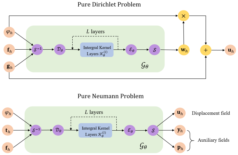
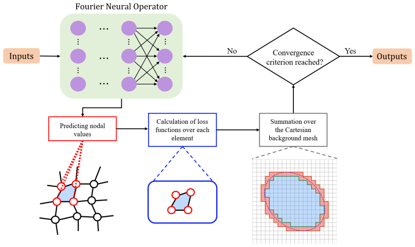
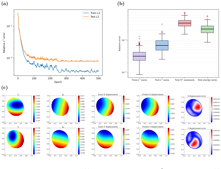
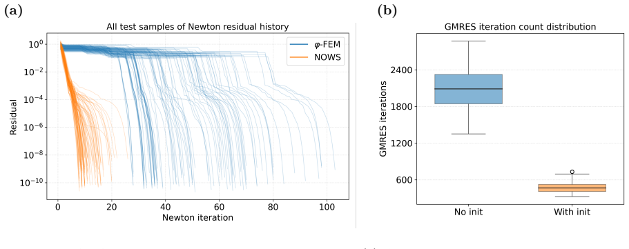
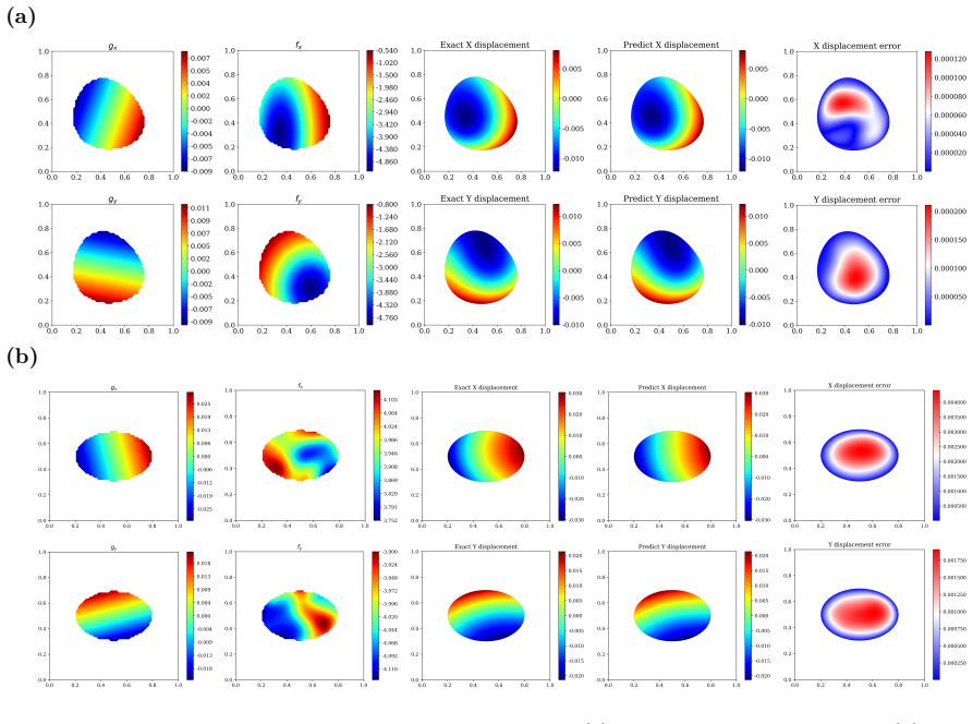
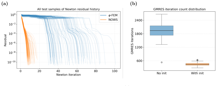
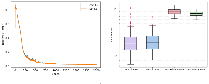
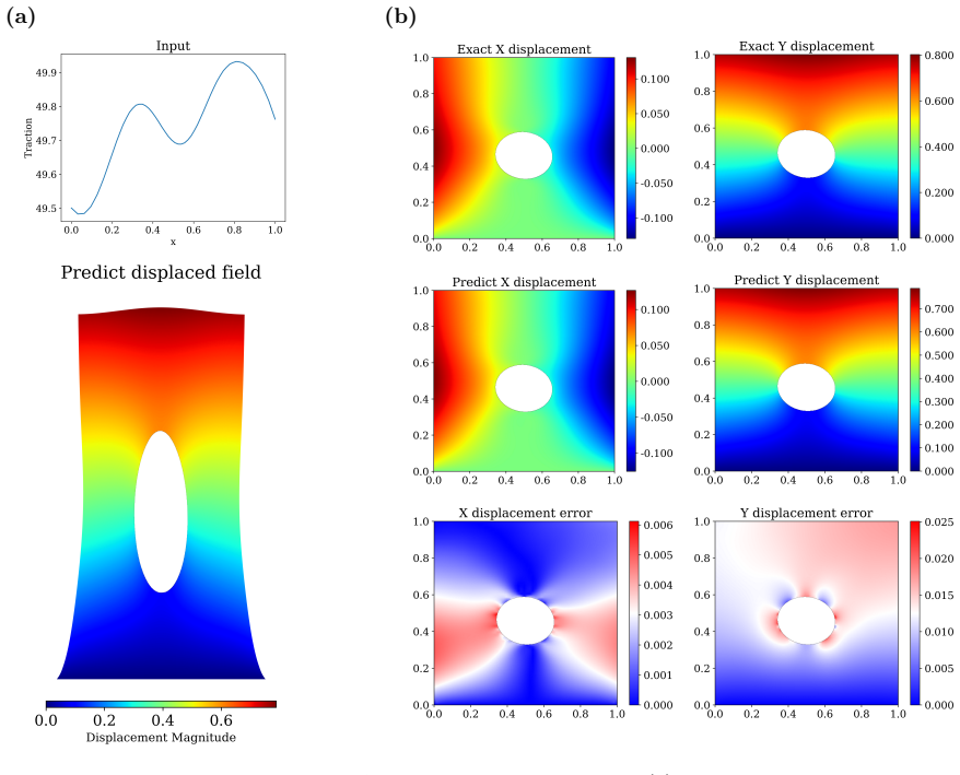
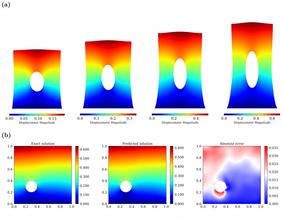
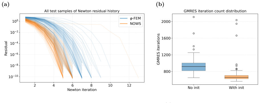
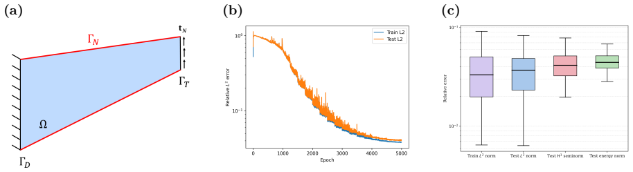
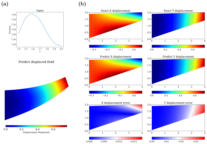
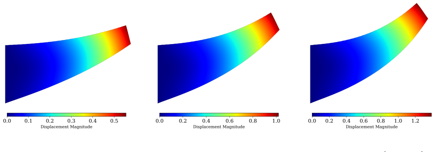
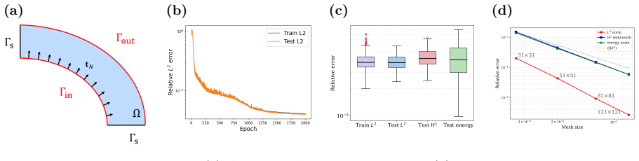
WINO is a neural operator whose parameters are obtained by minimizing the squared residuals of the weak form of the hyperelastic equations discretized with phi-FEM, together with squared penalties on the auxiliary equations that arise on cut cells. For Dirichlet problems only the homogeneous part of the displacement is learned via the phi-FEM lifting; for Neumann problems the network also outputs the auxiliary fields required by the unfitted formulation. Once trained, the operator produces displacement fields whose relative error stays below 0.04 on the reported benchmarks and supplies initial guesses that reduce the iteration count of nonlinear phi-FEM solvers.
What carries the argument
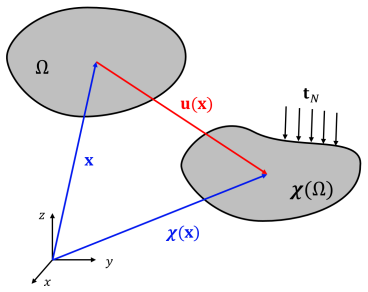
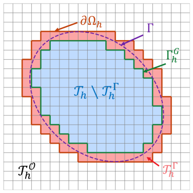
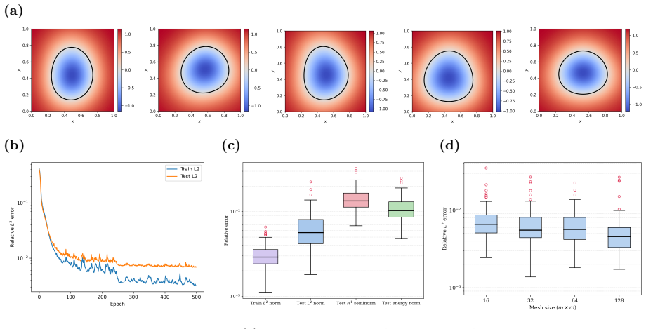
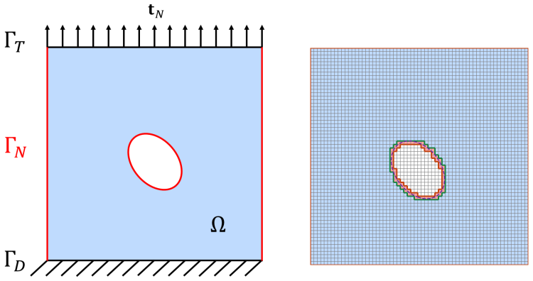
phi-FEM, the unfitted finite-element technique that represents arbitrary domain geometry by a level-set function on a fixed background mesh, allowing the weak residual of the governing equations to be evaluated directly as a training loss without body-fitted remeshing or reference solutions.
If this is right
- WINO produces solutions whose relative error is below 0.04 on all hyperelastic benchmarks without ever seeing paired reference data.
- Total wall-clock time for obtaining solutions drops by 50 to 80 percent relative to purely data-driven neural operators.
- Feeding WINO outputs as initial guesses into nonlinear phi-FEM solvers measurably reduces the number of iterations required for convergence.
- The same training procedure accommodates both Dirichlet and Neumann boundary conditions on domains whose shapes are encoded by level-set functions.
Where Pith is reading between the lines
- The residual-minimization strategy may transfer to other nonlinear constitutive laws once the corresponding weak form is written.
- Embedding the operator inside an outer optimization loop over geometry parameters could accelerate shape-design tasks that repeatedly solve hyperelastic problems.
Load-bearing premise
That penalizing the squared weak-form residuals of the phi-FEM discretization is sufficient to determine an accurate mapping from domain and load parameters to displacement fields without any supervised reference data.
What would settle it
Apply the trained WINO to a hyperelastic problem whose domain shape was withheld from training, compute the relative L2 error of the predicted displacement against a converged reference solution obtained by a body-fitted solver, and check whether the error remains below 0.04; an error above that threshold on multiple such cases would falsify the accuracy claim.
Figures

read the original abstract
We propose a Weak-form Physics-Informed Neural Operator (WINO), a data-free framework that combines the efficiency of neural operators with the geometric flexibility of the $\varphi$-finite element method ($\varphi$-FEM). $\varphi$-FEM is an unfitted method that accommodates geometric variations without body-fitted meshes, where the domain geometry is represented by the level-set function $\varphi$. To impose the boundary conditions, Dirichlet problems adopt the $\varphi$-FEM lifting so only the homogeneous displacement contribution is learned, whereas traction-driven Neumann problems additionally predict the auxiliary fields necessary for the unfitted weak formulation. Parameters are trained by minimizing squared weak-form residuals aligned with $\varphi$-FEM together with squared penalties on the cut-cell auxiliary equations, which removes the need for large paired datasets of converged reference solutions. After training, WINO outputs can seed the nonlinear $\varphi$-FEM solvers as neural operator warm starts (NOWS), which reduce iteration counts relative to traditional cold-started solvers. Numerical benchmarks show that WINO achieves high accuracy below 0.04 across all benchmarks, while reducing total computational time by 50--80\% compared with purely data-driven methods.
Editorial analysis
A structured set of objections, weighed in public.
Referee Report
Summary. The manuscript proposes WINO, a weak-form physics-informed neural operator for hyperelasticity on variable domains. It combines neural operators with the unfitted ϕ-FEM discretization (level-set geometry representation), trains data-free by minimizing squared weak-form residuals plus penalties on cut-cell auxiliary equations, and uses the resulting operator outputs as warm starts (NOWS) for nonlinear ϕ-FEM solvers. Benchmarks are claimed to reach errors below 0.04 with 50-80% total time reduction versus purely data-driven approaches.
Significance. If the data-free training via the composite weak-form loss is shown to be consistent for nonlinear hyperelasticity and to generalize across held-out level-set domains, the approach would offer a useful bridge between physics-informed operators and unfitted FEM, reducing reliance on paired reference data while accelerating nonlinear solves via warm starts.
major comments (2)
- [Abstract] Abstract: the central claim that minimizing squared weak-form residuals aligned with ϕ-FEM (plus cut-cell penalties) yields accurate solutions without any paired reference data rests on an unverified assumption that the true displacement is a global minimizer of the composite loss for nonlinear strain-energy functions; no derivation of consistency or analysis of spurious minima is provided.
- [Abstract] Abstract: the reported accuracy below 0.04 is not accompanied by any indication that the benchmarks were performed on held-out variable domains (rather than training geometries), which is required to substantiate the operator's generalization claim across level-set-defined domains.
minor comments (1)
- [Abstract] Abstract: the phrase 'high accuracy below 0.04' is imprecise without specifying the error measure (e.g., L2 or energy norm) or the precise benchmark problems.
Simulated Author's Rebuttal
We thank the referee for the constructive feedback on the theoretical justification and the need to clarify generalization in the benchmarks. We address each major comment below.
read point-by-point responses
-
Referee: [Abstract] Abstract: the central claim that minimizing squared weak-form residuals aligned with ϕ-FEM (plus cut-cell penalties) yields accurate solutions without any paired reference data rests on an unverified assumption that the true displacement is a global minimizer of the composite loss for nonlinear strain-energy functions; no derivation of consistency or analysis of spurious minima is provided.
Authors: We agree that the manuscript provides no formal derivation of consistency nor analysis of spurious minima for the nonlinear hyperelastic composite loss. The approach is motivated by the variational structure of the weak form (zero residual at the true solution) and is supported only by empirical results. We will revise the manuscript to add an explicit discussion of this assumption, its potential limitations for nonlinear problems, and references to related analyses in weak-form PINNs. revision: yes
-
Referee: [Abstract] Abstract: the reported accuracy below 0.04 is not accompanied by any indication that the benchmarks were performed on held-out variable domains (rather than training geometries), which is required to substantiate the operator's generalization claim across level-set-defined domains.
Authors: The full manuscript reports the accuracy below 0.04 on held-out level-set domains unseen during training, as detailed in the numerical experiments section. This detail is omitted from the abstract. We will revise the abstract to state explicitly that the reported accuracy holds on held-out variable domains. revision: yes
Circularity Check
No significant circularity; derivation grounded in external weak-form physics
full rationale
The paper's core training procedure minimizes squared residuals of the weak form taken directly from the established ϕ-FEM formulation (an unfitted method using level-set geometry), together with auxiliary penalties. This loss is defined by the PDE weak form and boundary conditions, which are independent inputs not derived from or fitted to the neural operator outputs. No equations reduce the claimed solution to a self-definition, a renamed fit, or a self-citation chain; the method is benchmarked against reference solutions on variable domains. The approach follows standard physics-informed operator learning and remains self-contained against external verification.
Axiom & Free-Parameter Ledger
axioms (1)
- domain assumption The weak form of the hyperelastic equations is a valid way to enforce the physics.
Reference graph
Works this paper leans on
-
[1]
Nonlinear solid mechanics: a continuum approach for engineering science,
G. A. Holzapfel, “Nonlinear solid mechanics: a continuum approach for engineering science,” 2002
2002
-
[2]
Topics in finite elasticity: hyperelasticity of rubber, elastomers, and biological tissues— with examples,
M. F. Beatty, “Topics in finite elasticity: hyperelasticity of rubber, elastomers, and biological tissues— with examples,” 1987
1987
-
[3]
O. C. Zienkiewicz, R. L. Taylor, P. Nithiarasu, and J. Zhu, The finite element method . Elsevier, 1977, vol. 3
1977
-
[4]
An introduction to the finite element method,
J. N. Reddy, “An introduction to the finite element method,” in Dynamics of Earth’s Fluid System . CRC Press, 2026, pp. 199–226
2026
-
[5]
Finite element implementation of incompressible, transversely isotropic hyperelasticity,
J. A. Weiss, B. N. Maker, and S. Govindjee, “Finite element implementation of incompressible, transversely isotropic hyperelasticity,” Computer methods in applied mechanics and engineering , vol. 135, no. 1-2, pp. 107–128, 1996
1996
-
[6]
J. W. Thomas, Numerical partial differential equations: finite difference methods . Springer Science & Business Media, 2013, vol. 22
2013
-
[7]
L. Lu, P. Jin, and G. E. Karniadakis, “Deeponet: Learning nonlinear operators for identifying differential equations based on the universal approximation theorem of operators,” arXiv preprint arXiv:1910.03193, 2019
work page internal anchor Pith review Pith/arXiv arXiv 1910
-
[8]
Learning nonlinear operators via deeponet based on the universal approximation theorem of operators,
L. Lu, P. Jin, G. Pang, Z. Zhang, and G. E. Karniadakis, “Learning nonlinear operators via deeponet based on the universal approximation theorem of operators,” Nature machine intelligence , vol. 3, no. 3, pp. 218–229, 2021
2021
-
[9]
Fourier Neural Operator for Parametric Partial Differential Equations
Z. Li, N. Kovachki, K. Azizzadenesheli, B. Liu, K. Bhattacharya, A. Stuart, and A. Anand- kumar, “Fourier neural operator for parametric partial differential equations,” arXiv preprint arXiv:2010.08895, 2020
work page internal anchor Pith review Pith/arXiv arXiv 2010
-
[10]
Synergistic learning with multi-task deeponet for efficient pde problem solving,
V. Kumar, S. Goswami, K. Kontolati, M. D. Shields, and G. E. Karniadakis, “Synergistic learning with multi-task deeponet for efficient pde problem solving,” Neural Networks , vol. 184, p. 107113, 2025. 37
2025
-
[11]
Physics-informed neural operator for learning partial differential equations,
Z. Li, H. Zheng, N. Kovachki, D. Jin, H. Chen, B. Liu, K. Azizzadenesheli, and A. Anandkumar, “Physics-informed neural operator for learning partial differential equations,” ACM/IMS Journal of Data Science , vol. 1, no. 3, pp. 1–27, 2024
2024
-
[12]
Learning the solution operator of parametric partial dif- ferential equations with physics-informed deeponets,
S. Wang, H. Wang, and P. Perdikaris, “Learning the solution operator of parametric partial dif- ferential equations with physics-informed deeponets,” Science advances, vol. 7, no. 40, p. eabi8605, 2021
2021
-
[13]
Physics-informed machine learning in biomedical science and engineering,
N. Ahmadi, Q. Cao, J. D. Humphrey, and G. E. Karniadakis, “Physics-informed machine learning in biomedical science and engineering,” Annual Review of Biomedical Engineering , vol. 28, no. 1, pp. 309–336, 2026
2026
-
[14]
Variational physics-informed neural operator (vino) for solving partial differential equations,
M. S. Eshaghi, C. Anitescu, M. Thombre, Y. Wang, X. Zhuang, and T. Rabczuk, “Variational physics-informed neural operator (vino) for solving partial differential equations,” Computer Methods in Applied Mechanics and Engineering , vol. 437, p. 117785, 2025
2025
-
[15]
Finite element operator network for solving parametric pdes,
J. Y. Lee, S. Ko, and Y. Hong, “Finite element operator network for solving parametric pdes,” arXiv preprint arXiv:2308.04690 , 2023
-
[16]
NOWS: Neural Operator Warm Starts for Accelerating Iterative Solvers
M. S. Eshaghi, C. Anitescu, N. Valizadeh, Y. Wang, X. Zhuang, and T. Rabczuk, “Nows: Neural operator warm starts for accelerating iterative solvers,” arXiv preprint arXiv:2511.02481 , 2025
work page internal anchor Pith review Pith/arXiv arXiv 2025
-
[17]
Y. Wang, Z. Hao, M. S. Eshaghi, C. Anitescu, X. Zhuang, T. Rabczuk, and Y. Liu, “Pretrain finite element method: A pretraining and warm-start framework for pdes via physics-informed neural operators,” arXiv preprint arXiv:2601.03086 , 2026
-
[18]
Level set methods: an overview and some recent results,
S. Osher and R. P. Fedkiw, “Level set methods: an overview and some recent results,” Journal of Computational physics , vol. 169, no. 2, pp. 463–502, 2001
2001
-
[19]
Level set methods and dynamic implicit surfaces,
S. Osher, R. Fedkiw, and K. Piechor, “Level set methods and dynamic implicit surfaces,” Appl. Mech. Rev., vol. 57, no. 3, pp. B15–B15, 2004
2004
-
[20]
ϕ-fem: a finite element method on domains defined by level-sets,
M. Duprez and A. Lozinski, “ ϕ-fem: a finite element method on domains defined by level-sets,” SIAM Journal on Numerical Analysis , vol. 58, no. 2, pp. 1008–1028, 2020
2020
-
[21]
φ-fem, a finite element method on domains defined by level-sets: the neumann boundary case,
M. Duprez, V. Lleras, and A. Lozinski, “ φ-fem, a finite element method on domains defined by level-sets: the neumann boundary case,” 2020
2020
-
[22]
φ-fem-fno: a new approach to train a neural operator as a fast pde solver for variable geometries,
M. Duprez, V. Lleras, A. Lozinski, V. Vigon, and K. Vuillemot, “ φ-fem-fno: a new approach to train a neural operator as a fast pde solver for variable geometries,” Communications in Nonlinear Science and Numerical Simulation , p. 109131, 2025
2025
-
[23]
Cut finite element methods,
E. Burman, P. Hansbo, M. G. Larson, and S. Zahedi, “Cut finite element methods,” Acta Numerica, vol. 34, pp. 1–121, 2025
2025
-
[24]
Bonet and R
J. Bonet and R. D. Wood, Nonlinear continuum mechanics for finite element analysis . Cambridge university press, 1997
1997
-
[25]
C. T. Kelley, Solving nonlinear equations with Newton ’s method . SIAM, 2003
2003
-
[26]
Nitsol: A newton iterative solver for nonlinear systems,
M. Pernice and H. F. Walker, “Nitsol: A newton iterative solver for nonlinear systems,” SIAM Journal on Scientific Computing , vol. 19, no. 1, pp. 302–318, 1998. 38
1998
-
[27]
Function minimization by conjugate gradients,
R. Fletcher and C. M. Reeves, “Function minimization by conjugate gradients,” The computer journal, vol. 7, no. 2, pp. 149–154, 1964
1964
-
[28]
A survey of nonlinear conjugate gradient methods,
W. W. Hager and H. Zhang, “A survey of nonlinear conjugate gradient methods,” Pacific journal of Optimization, vol. 2, no. 1, pp. 35–58, 2006
2006
-
[29]
Gmres: A generalized minimal residual algorithm for solving non- symmetric linear systems,
Y. Saad and M. H. Schultz, “Gmres: A generalized minimal residual algorithm for solving non- symmetric linear systems,” SIAM Journal on scientific and statistical computing , vol. 7, no. 3, pp. 856–869, 1986
1986
-
[30]
Gmres with deflated restarting,
R. B. Morgan, “Gmres with deflated restarting,” SIAM Journal on Scientific Computing , vol. 24, no. 1, pp. 20–37, 2002
2002
-
[31]
Petsc users manual,
S. Balay, S. Abhyankar, M. Adams, J. Brown, P. Brune, K. Buschelman, L. Dalcin, A. Dener, V. Eijkhout, W. Gropp et al. , “Petsc users manual,” 2019
2019
-
[32]
SOAP: Improving and Stabilizing Shampoo using Adam
N. Vyas, D. Morwani, R. Zhao, M. Kwun, I. Shapira, D. Brandfonbrener, L. Janson, and S. Kakade, “Soap: Improving and stabilizing shampoo using adam,” arXiv preprint arXiv:2409.11321 , 2024
work page internal anchor Pith review Pith/arXiv arXiv 2024
-
[33]
Gaussian processes in machine learning,
C. E. Rasmussen, “Gaussian processes in machine learning,” in Summer school on machine learning . Springer, 2003, pp. 63–71
2003
-
[34]
G. H. Golub and C. F. Van Loan, Matrix computations . JHU press, 2013. 39
2013
discussion (0)
Sign in with ORCID, Apple, or X to comment. Anyone can read and Pith papers without signing in.