Revealing the Two-Fold Ambiguity: Tau Momentum Reconstruction and Its Impact on Entanglement Observables
Pith reviewed 2026-06-29 17:21 UTC · model grok-4.3
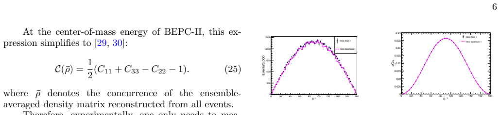
The pith
Kinematic constraints in tau-pair events allow reconstruction of two possible momenta, yet entanglement signals remain extractable even without identifying the true solution.
A machine-rendered reading of the paper's core claim, the machinery that carries it, and where it could break.
Core claim
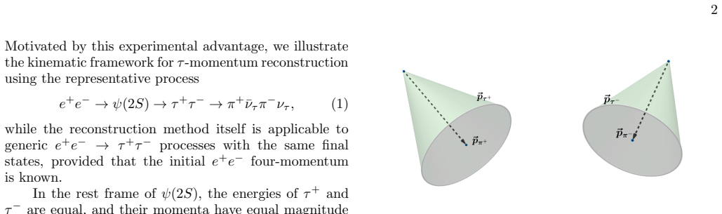
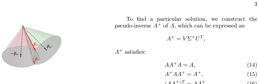
For the process e+e− → τ+τ− → π+ ν¯τ π− ντ, the kinematic constraints allow the τ momenta to be reconstructed up to a well-known two-fold ambiguity, regardless of the presence of an intermediate resonance state. A geometric interpretation of the ambiguity is presented together with a numerical reconstruction method based on singular value decomposition. Using only the information from visible final-state particles and decay kinematics, the method reconstructs the two possible solutions for the τ+τ− pair. Monte Carlo simulations in typical collider environments validate the reconstruction performance, and the impact on spin-entanglement measurements is shown to leave reliable signals extracta
What carries the argument
The two-fold kinematic ambiguity arising from the missing neutrinos, located geometrically and solved numerically by singular value decomposition on the visible pion four-momenta and decay constraints.
If this is right
- The reconstruction succeeds for any intermediate resonance state in the tau decay chain.
- The SVD-based procedure supplies both candidate solutions from visible particles alone.
- Entanglement observables computed from the mixed solutions still yield detectable signals.
- The approach supplies a practical tool for tau kinematics and entanglement studies at e+e− colliders.
Where Pith is reading between the lines
- The same two-fold structure may appear in other missing-energy final states, suggesting the SVD method could be tested on additional decay channels.
- If the ambiguity persists across different center-of-mass energies, the technique could be applied directly to existing collider datasets without new hardware.
- The result implies that partial kinematic information is often sufficient for quantum-correlation measurements, opening the possibility of studying entanglement in processes with more complex missing particles.
Load-bearing premise
The kinematic constraints from visible particles and decay kinematics always produce exactly two reconstructible solutions for the tau momenta, independent of any intermediate resonance, and Monte Carlo simulations faithfully represent the reconstruction and entanglement extraction that would occur in real data.
What would settle it
A Monte Carlo study in which the entanglement observable extracted after randomly mixing true and spurious solutions falls below statistical significance while the same observable computed from the true solutions alone remains clearly nonzero.
Figures
read the original abstract
The neutrinos produced in $\tau$ decays cannot be directly detected, making the reconstruction of $\tau$ kinematics challenging and affecting measurements of quantum correlations such as spin entanglement. For the process $e^+e^- \to \tau^+\tau^- \to \pi^+ \bar{\nu}_\tau\pi^-\nu_\tau$, the kinematic constraints allow the $\tau$ momenta to be reconstructed up to a well-known two-fold ambiguity, regardless of the presence of an intermediate resonance state. In this paper, we present a geometric interpretation of this ambiguity and propose a numerical reconstruction method based on singular value decomposition (SVD). Using only the information from visible final-state particles and decay kinematics, the method reconstructs the two possible solutions for the $\tau^+\tau^-$ pair. The reconstruction performance is validated with Monte Carlo simulations in typical collider environments. We further investigate the impact of the spurious solution on spin-entanglement measurements and show that reliable entanglement signals can still be extracted even when the true and spurious solutions cannot be experimentally distinguished. This work provides a practical approach for $\tau$-lepton kinematic reconstruction and spin-entanglement measurements in $e^+e^-$ collider experiments.
Editorial analysis
A structured set of objections, weighed in public.
Referee Report
Summary. The paper claims that for e+e− → τ+τ− → π+ ν̄τ π− ντ, kinematic constraints from visible pions and beam four-momentum yield a two-fold ambiguity in τ momenta reconstruction independent of intermediate resonances. It provides a geometric interpretation, proposes an SVD-based numerical method to recover both solutions from visible particles alone, validates performance via Monte Carlo in collider environments, and shows that spin-entanglement observables remain extractable even when true and spurious solutions cannot be distinguished experimentally.
Significance. If the reconstruction method is shown to reliably recover both quadratic roots and the MC validation includes quantitative metrics on accuracy and entanglement bias, the work would provide a practical tool for τ kinematic reconstruction at e+e− colliders, enabling more robust quantum correlation studies. The explicit treatment of the ambiguity and its impact on entanglement is a positive contribution, though the absence of detailed performance numbers in the abstract limits immediate assessment of robustness.
major comments (2)
- [§3] §3 (reconstruction method) and Eq. (derived from p_τ² = m_τ² after neutrino elimination): the SVD procedure is presented as recovering both solutions of the quadratic ambiguity, but SVD applies to linear systems; the manuscript must explicitly demonstrate that the linear subsystem is isolated and the remaining quadratic is solved analytically (or that the numerical SVD recovers both physical roots) rather than returning a single or unphysical solution. This is load-bearing for the central claim of reconstructing 'the two possible solutions' from visible particles alone.
- [§4] §4 (Monte Carlo validation): no quantitative performance metrics (e.g., efficiency for both solutions, resolution on reconstructed p_τ, or fraction of events where the spurious solution is selected) or error analysis are provided to support the assertion that 'reliable entanglement signals can still be extracted'; without these, the robustness claim cannot be evaluated.
minor comments (2)
- [Abstract] Abstract: the statement 'regardless of the presence of an intermediate resonance state' should be supported by an explicit check or reference to a section showing the quadratic structure is unchanged.
- [§3] Notation: define the SVD matrix construction and the quadratic variable clearly in the first appearance to avoid ambiguity for readers unfamiliar with the kinematic setup.
Simulated Author's Rebuttal
We thank the referee for the detailed and constructive report. We address the two major comments point by point below. Both points identify areas where the manuscript presentation can be strengthened, and we will revise accordingly.
read point-by-point responses
-
Referee: [§3] §3 (reconstruction method) and Eq. (derived from p_τ² = m_τ² after neutrino elimination): the SVD procedure is presented as recovering both solutions of the quadratic ambiguity, but SVD applies to linear systems; the manuscript must explicitly demonstrate that the linear subsystem is isolated and the remaining quadratic is solved analytically (or that the numerical SVD recovers both physical roots) rather than returning a single or unphysical solution. This is load-bearing for the central claim of reconstructing 'the two possible solutions' from visible particles alone.
Authors: We agree that §3 would benefit from an explicit step-by-step isolation of the linear constraints before applying SVD, followed by the analytic solution of the remaining quadratic. In the revised manuscript we will add a dedicated subsection that (i) writes the full set of kinematic equations, (ii) separates the linear subsystem in the unknown neutrino four-momenta, (iii) shows how the SVD of the associated matrix yields the two-dimensional null space, and (iv) substitutes back into the quadratic mass-shell condition to obtain the two physical roots. This will be illustrated with the explicit matrix forms and a short numerical example confirming both roots are recovered. revision: yes
-
Referee: [§4] §4 (Monte Carlo validation): no quantitative performance metrics (e.g., efficiency for both solutions, resolution on reconstructed p_τ, or fraction of events where the spurious solution is selected) or error analysis are provided to support the assertion that 'reliable entanglement signals can still be extracted'; without these, the robustness claim cannot be evaluated.
Authors: We accept that the current Monte Carlo section lacks the quantitative figures needed to substantiate the robustness claim. In the revision we will augment §4 with tables and plots reporting (a) the fraction of events for which both solutions are successfully reconstructed, (b) the momentum resolution (RMS and bias) for the true versus spurious solutions, (c) the fraction of events in which the spurious solution is closer to the true momentum, and (d) the bias and uncertainty on the extracted entanglement observables when the two solutions are averaged or randomly selected. Error propagation from the SVD singular values will also be included. revision: yes
Circularity Check
No significant circularity: reconstruction follows directly from kinematic constraints
full rationale
The paper's central claim rests on applying four-momentum conservation and on-shell conditions (p_τ² = m_τ², p_ν² = 0) to visible decay products, which algebraically produces a known quadratic equation whose two roots constitute the documented two-fold ambiguity. The SVD step is presented as a numerical solver for the resulting linear subsystem after neutrino elimination; no parameter is fitted to data and then relabeled as a prediction, and no self-citation chain is invoked to justify uniqueness or the functional form. Monte Carlo validation is an external consistency check, not an input that defines the output. The derivation chain therefore remains self-contained and does not reduce to its own assumptions by construction.
Axiom & Free-Parameter Ledger
Reference graph
Works this paper leans on
-
[1]
Similarly forA T A, obtained are the eigenvaluesλ 1,λ 2, λ3 and their corresponding eigenvectorsv 1,v 2,v 3, which form the matrixV: V= v1 v2 v3
Singular Value Decomposition (SVD) Framework By virtue of SVD, the matrixAcan be decomposed into three matrices [22, 23]: A=UΣV T ,(13) whereUis a 2×2 square matrix, Σ is a 2×3 matrix, andV T is a 3×3 matrix.UandVare constructed from Aas follows: forAA T : obtained are the eigenvaluesλ 1 andλ 2 with corresponding eigenvectorsu 1 andu 2, which form the mat...
-
[2]
Unit Norm Constraint and the Number of Solutions For the general solution, we require it to be a unit vector (i.e.,|ˆu|2 = 1). This translates the general solution into a quadratic equation inα: α2|v3|2 + 2α(u0 ·v 3) + (|u0|2 −1) = 0,(20) The discriminant of the above equation is: ∆ = 4 (u0 ·v 3)2 − |v3|2(|u0|2 −1) .(21) If ∆>0, the equation has two real ...
-
[3]
Reconstruction Procedure
-
[4]
Construct the four-momenta from the visible par- ticles
-
[5]
Construct the constraint matrixAand vectorb
-
[6]
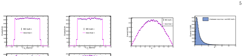
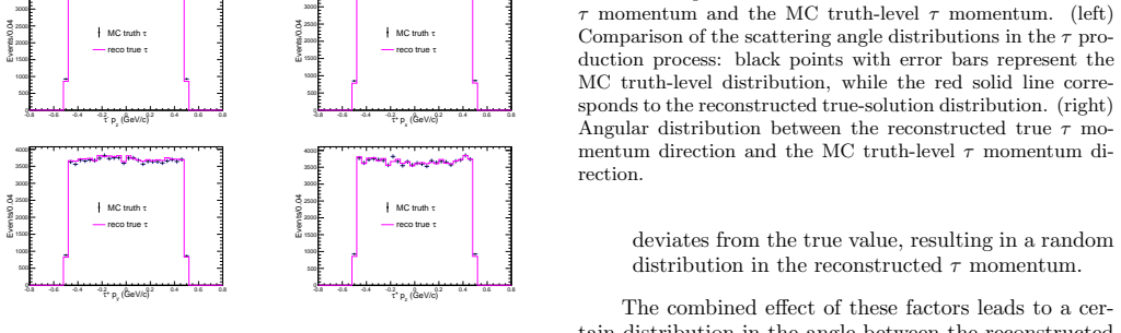
For each event, solve using SVD to obtain theτ momentum. III. MONTE CARLO SIMULATION AND VALIDATION A. Simulation Setup To verify the accuracy of the SVD method in recon- structingτ +τ −, we perform numerical experiments us- ing Monte Carlo simulation software. For simplification, we only consider two important experimental parame- ters: the energy spread...
-
[7]
MC truth-level
the trueτ +τ − (“MC truth-level” data)
-
[8]
MC truth-level
the momentum information of the visible decay productsπ + andπ −. B. Reconstruction Efficiency Statistics Based on the kinematic information ofπ + andπ −, theτmomentum direction is reconstructed using the SVD method. Table I summarises the reconstruction statistics for 1×10 5 simulated events. When beam en- ergy spread and detector resolution are included...
2000
-
[9]
true solution
Treatment Of the Two-fold Ambiguity Among the Two-fold Ambiguity arising from the re- construction process, besides the “true solution” corre- sponding to the actual physical process, the other solu- tion also strictly satisfies the four-momentum conserva- tion of theτdecay. This solution is kinematically self- consistent and can be regarded as another po...
2000
-
[10]
Entanglement Analysis with the Two-fold Ambiguity The experimental procedure is as follows:
-
[11]
Input the three-momenta ofπ + andπ −
-
[12]
Obtain the four-momenta ofτ + andτ − (retaining both solutions)
-
[13]
Compute the correlation matrixC ij and concur- rence estimatorC(θ i, βi) of each event
-
[14]
Figure 5 presents a comparison of the concurrence distributions computed from the true-solution set and the spurious-solution set
Compute the concurrence as 1 C(¯ρ) =⟨C(θ, β)⟩= 1 N NX i=1 C(θi, βi).(27) Following the above procedure, we obtain the entangle- ment results for the three datasets. Figure 5 presents a comparison of the concurrence distributions computed from the true-solution set and the spurious-solution set. As can be seen from the figure, the two distributions are in ...
-
[15]
The fine-structure constant is denoted byα=e 2/4π
Total Cross Section and Interference The Born cross section fore +e− →τ +τ − is de- scribed by the coherent sum of a continuum amplitude (virtual photon exchange) and a resonance amplitude (ψ(2S)): σ(s) = s 12π e2 s + gV,τ gV,e s−m 2 V +im V ΓV 2 β 1 + 2m2 τ s , wheresis the squared center-of-mass (c.m.) energy,m V and ΓV [32] are the mass and total width...
-
[16]
Energy with Beam Spread The beam energy spread of BEPC-II is approxi- mately Gaussian with widthσ E = 1.2 MeV
Sampling of the c.m. Energy with Beam Spread The beam energy spread of BEPC-II is approxi- mately Gaussian with widthσ E = 1.2 MeV. For each event the actual c.m. energyWis sampled as W=W 0 +σ E ·ξ, ξ∼ N(0,1), 8 TABLE II. Comparison of the mean concurrence⟨C⟩(mean±stat.) among the MC truth, true solution, and spurious solution in differentθbins θbin (deg)...
-
[17]
frame, the direction of theτ − is charac- terized by the polar angleθrelative to the electron beam axis
Angular Distribution and Polarization inτ +τ − Production In the c.m. frame, the direction of theτ − is charac- terized by the polar angleθrelative to the electron beam axis. The normalized angular distribution is given by the QED formula (including theτmass effect): 1 σ dσ dcosθ ∝1 + cos 2 θ+ 4m2 τ s sin2 θ. The azimuthal angleϕis uniformly distributed i...
-
[18]
In the rest frame of theτ, the decay is two- body; the pion energy is fixed: Erest π = m2 τ +m 2 π 2mτ , p rest π = p (Erestπ )2 −m 2π
Decay ofτLeptons to pions Only the decaysτ − →π −ντ andτ + →π +¯ντ are simulated. In the rest frame of theτ, the decay is two- body; the pion energy is fixed: Erest π = m2 τ +m 2 π 2mτ , p rest π = p (Erestπ )2 −m 2π. The angular distribution of the pion with respect to theτpolarization direction is linear due to theV−A interaction: dΓ dcosθ π ∝1 +α πPτ c...
-
[19]
If theτhas four- momentum (Eτ , ⃗ pτ) in the lab frame, then the boost ve- locity is ⃗β=⃗ pτ /Eτ andγ=E τ /mτ
Lorentz Transformation to the Laboratory Frame The four-momentum of the pion in the labora- tory frame is obtained by boosting the rest-frame four- momentum with theτvelocity. If theτhas four- momentum (Eτ , ⃗ pτ) in the lab frame, then the boost ve- locity is ⃗β=⃗ pτ /Eτ andγ=E τ /mτ. The lab-frame pion four-momentum is Elab π =γ Erest π + ⃗β·⃗ prest π ,...
-
[20]
Y. Afik and J. R. M. de Nova, Eur. Phys. J. Plus136, 907 (2021), arXiv:2003.02280 [quant-ph]
-
[21]
M. Fabbrichesi, R. Floreanini, and G. Panizzo, Phys. Rev. Lett.127, 161801 (2021), arXiv:2102.11883 [hep- ph]
- [22]
- [23]
-
[24]
Y. Afik and J. R. M. de Nova, Quantum6, 820 (2022), arXiv:2203.05582 [quant-ph]
- [25]
-
[26]
M. Fabbrichesi, R. Floreanini, and E. Gabrielli, Eur. Phys. J. C83, 162 (2023), arXiv:2208.11723 [hep-ph]
-
[27]
C. Severi and E. Vryonidou, JHEP01, 148 (2023), arXiv:2210.09330 [hep-ph]
- [28]
- [29]
-
[30]
Aadet al.(ATLAS), Nature633, 542 (2024), arXiv:2311.07288 [hep-ex]
G. Aadet al.(ATLAS), Nature633, 542 (2024), arXiv:2311.07288 [hep-ex]
-
[31]
A. Hayrapetyanet al.(CMS), Rept. Prog. Phys.87, 117801 (2024), arXiv:2406.03976 [hep-ex]
-
[32]
Ablikimet al.(BESIII), Nature Commun.16, 4948 (2025), arXiv:2505.14988 [hep-ex]
M. Ablikimet al.(BESIII), Nature Commun.16, 4948 (2025), arXiv:2505.14988 [hep-ex]
-
[33]
Privitera, Phys
P. Privitera, Phys. Lett. B288, 227 (1992)
1992
-
[34]
S. A. Abel, M. Dittmar, and H. K. Dreiner, Phys. Lett. B280, 304 (1992)
1992
-
[35]
H. K. Dreiner, in2nd Workshop on Tau Lepton Physics (1992) arXiv:hep-ph/9211203
work page internal anchor Pith review Pith/arXiv arXiv 1992
-
[36]
M. Fabbrichesi and L. Marzola, Phys. Rev. D110, 076004 (2024), arXiv:2405.09201 [hep-ph]
- [37]
-
[38]
M. Ablikimet al.(BESIII), Chin. Phys. C44, 040001 (2020), arXiv:1912.05983 [hep-ex]
- [39]
-
[40]
Precision Measurement of the Mass of the $\tau$ Lepton
M. Ablikimet al.(BESIII), Phys. Rev. D90, 012001 (2014), arXiv:1405.1076 [hep-ex]
work page internal anchor Pith review Pith/arXiv arXiv 2014
-
[41]
R. A. Sadek, (IJACSA) International Journal of Ad- vanced Computer Science and Applications3, 26 (2012), arXiv:1211.7102 [cs.CV]
work page internal anchor Pith review Pith/arXiv arXiv 2012
-
[42]
D. L. Lieven, D. M. Bart, and V. Joos, SIAM J. Matrix Anal. Appl.21, 1253 (2006)
2006
-
[43]
BEPC II Collaboration,Preliminary Design Report of accelerator BEPC II, Tech. Rep. (Institute of High En- ergy Physics, Chinese Academy of Sciences, 2003) sec- ond version, in Chinese;http://acc-center.ihep.ac. cn/bepcii/bepcii.htm
2003
-
[44]
Yuan, B.-Y
C.-Z. Yuan, B.-Y. Zhang, and Q. Qin, Chinese Physics C34, 1707 (2010), in Chinese
2010
-
[45]
BESIII Collaboration,Preliminary Design Report: The BESIII Detector, Tech. Rep. (Institute of High Energy Physics, Chinese Academy of Sciences, 2004)
2004
-
[46]
Fano, Rev
U. Fano, Rev. Mod. Phys.55, 855 (1983)
1983
-
[47]
W. K. Wootters, Phys. Rev. Lett.80, 2245 (1998), arXiv:quant-ph/9709029
work page internal anchor Pith review Pith/arXiv arXiv 1998
- [48]
- [49]
-
[50]
K. Ehat¨ aht, M. Fabbrichesi, L. Marzola, and C. Veelken, Phys. Rev. D109, 032005 (2024), arXiv:2311.17555 [hep- ph]
-
[51]
Navaset al.(Particle Data Group), Phys
S. Navaset al.(Particle Data Group), Phys. Rev. D110, 030001 (2024)
2024
-
[52]
M. N. Achasov, X. H. Mo, N. Y. Muchnoi, I. B. Nikolaev, S. A. Privalov, and J. Y. Zhang (BES-III), EPJ Web Conf.212, 08005 (2019)
2019
discussion (0)
Sign in with ORCID, Apple, or X to comment. Anyone can read and Pith papers without signing in.