Fewer simulations, sharper covariances: Reducing mock covariance noise with Zeldovich approximation control variates
Pith reviewed 2026-06-29 10:13 UTC · model grok-4.3
The pith
Pairing each mock simulation with a cheap Zeldovich approximation realization sharing the same initial conditions reduces the variance of the power spectrum covariance matrix estimate by roughly an order of magnitude on large scales.
A machine-rendered reading of the paper's core claim, the machinery that carries it, and where it could break.
Core claim
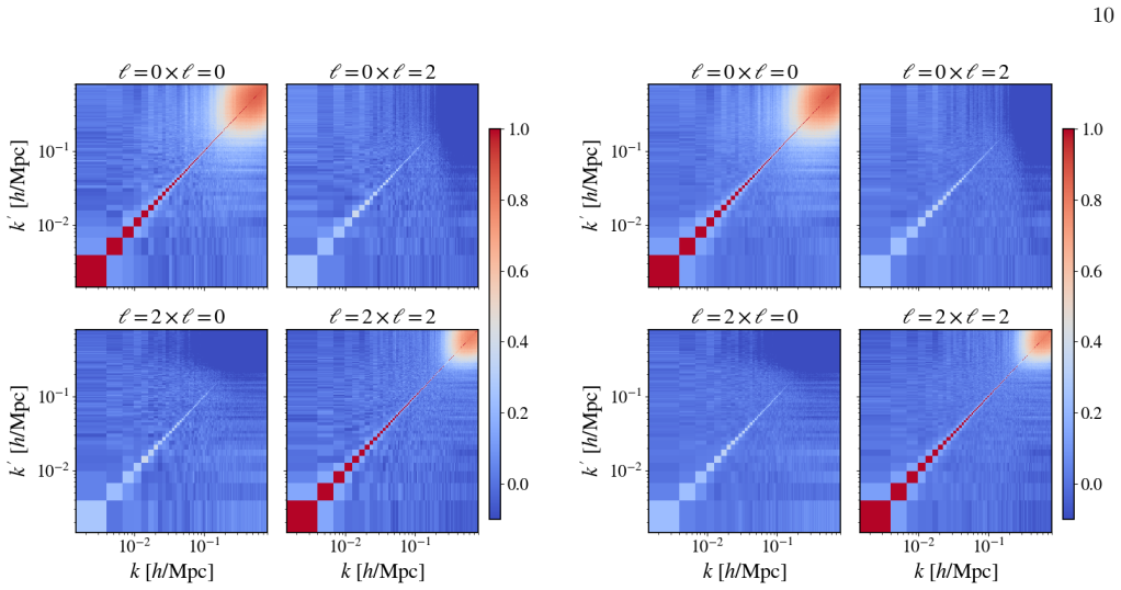
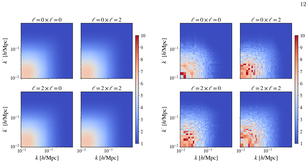
By pairing each target mock simulation with a Zeldovich-approximation realization that shares the identical initial conditions, the control-variate estimator removes correlated sample variance from the covariance matrix estimate. Under a Gaussian disconnected approximation the optimal coefficient beta and the resulting correlation rho are given by closed-form expressions involving only the auto- and cross-power spectra. For the monopole the correlation simplifies to the product of the squared cross-correlation coefficients at the two wavenumbers. On DESI-like mocks the method reduces covariance variance by roughly an order of magnitude for wavenumbers below 0.05 h per Mpc and by a factor of
What carries the argument
Zeldovich control variate: a cheap, initial-condition-matched realization whose known statistical properties are used to subtract correlated noise from the target covariance estimator.
If this is right
- The largest gains occur precisely on the large scales where covariance estimation is most difficult.
- The computational cost of obtaining accurate covariances drops by a factor of several for typical survey analyses.
- The analytic expressions allow the expected improvement to be calculated in advance from the cross-power spectrum alone.
- The method applies immediately to power-spectrum analyses in imaging and spectroscopic surveys.
Where Pith is reading between the lines
- The same pairing idea could be tested on other two-point or higher-order statistics where sample variance is also limiting.
- Once the cross-correlation coefficient is measured, the expected variance reduction can be forecasted without additional simulations.
- Extending the approach to multiple control variates of increasing fidelity might yield further gains at modest extra cost.
Load-bearing premise
The target mocks and their Zeldovich counterparts must share a sufficiently large fraction of their sample variance for the subtraction to produce a substantial reduction in estimator noise.
What would settle it
If the measured variance of the covariance-matrix elements obtained from an ensemble of paired mocks equals the variance obtained from the same number of unpaired mocks, the claimed reduction would be falsified.
Figures
read the original abstract
We present a control-variate method for reducing the variance of power spectrum covariance matrix estimates from simulations of large-scale structure. The key idea is to pair each mock simulation with a cheap Zeldovich-approximation realization sharing the same initial conditions, and to use the known statistical properties of the Zeldovich field to remove correlated sample variance from the covariance estimator. Under a Gaussian disconnected approximation, we derive fully analytic expressions for both the optimal control-variate coefficient, $\beta(k,\ell;k',\ell')$, and the corresponding correlation, $\rho(k,\ell;k',\ell')$, in terms of the auto- and cross-power spectra of the target and control fields. In the monopole case, the correlation takes the particularly simple form $\rho(k,k') = r^2(k),r^2(k')$, where $r(k)$ is the standard cross-correlation coefficient between the target and Zeldovich fields, implying that covariance estimation remains highly efficient whenever the two fields are strongly correlated. For masked redshift-space lognormal mocks, resembling Luminous Red Galaxies from the Dark Energy Spectroscopic Instrument (DESI), we find that the control-variate estimator reduces the variance of the covariance matrix by approximately an order of magnitude on large scales, $k \lesssim 0.05\,h\,{\rm Mpc}^{-1}$, precisely where accurate covariance estimation is most challenging. The gains are smaller for higher $k$ but typically accelerate convergence by a factor of 2-3, substantially lowering the computational cost of covariance estimation for current and upcoming large-scale structure surveys. Due to its simplicity, this method is readily implementable in current imaging and spectroscopic surveys (e.g., DESI, Euclid, LSST, PFS, SPHEREx).
Editorial analysis
A structured set of objections, weighed in public.
Referee Report
Summary. The paper presents a control-variate method for reducing variance in power-spectrum covariance estimates from large-scale structure mocks. Each full mock is paired with a cheap Zeldovich-approximation realization sharing the same initial conditions; under a Gaussian disconnected approximation, fully analytic expressions are derived for the optimal coefficient β(k,ℓ;k',ℓ') and the correlation ρ(k,ℓ;k',ℓ'). In the monopole this reduces to ρ(k,k')=r²(k)r²(k'), where r(k) is the cross-correlation coefficient between target and Zeldovich fields. Tests on masked redshift-space lognormal mocks resembling DESI LRGs report an order-of-magnitude reduction in covariance-matrix variance for k≲0.05 h Mpc^{-1} and factors of 2–3 at higher k.
Significance. If the gains generalize, the approach would materially lower the number of expensive simulations required for accurate covariance estimation in ongoing and future surveys. The provision of closed-form expressions for β and ρ, together with the especially simple monopole result, constitutes a clear technical strength that distinguishes the work from purely numerical control-variate schemes.
major comments (2)
- [Numerical results (lognormal-mock tests)] The central empirical result—an approximately order-of-magnitude reduction in covariance variance for k≲0.05 h Mpc^{-1}—is obtained exclusively from lognormal mocks. Because these fields contain weaker mode coupling and connected four-point contributions than N-body realizations, both the cross-correlation r(k) with the Zeldovich control field and the accuracy of the Gaussian disconnected approximation used to fix β may be systematically higher than would occur in the target application; this directly affects the load-bearing claim that the method substantially lowers computational cost for surveys such as DESI.
- [Analytic derivation of β and ρ] The derivation of β(k,ℓ;k',ℓ') and ρ(k,ℓ;k',ℓ') is performed under the Gaussian disconnected approximation. The manuscript does not quantify the residual bias or variance inflation that arises when connected non-Gaussian terms are restored, nor does it test whether the analytic β remains near-optimal once those terms are present; this approximation is load-bearing for the claimed analytic simplicity and efficiency.
minor comments (1)
- [Numerical results] A short paragraph describing the precise masking and redshift-space distortion implementation applied to the lognormal fields would improve reproducibility of the reported gains.
Simulated Author's Rebuttal
We thank the referee for the positive summary and constructive major comments. We respond to each point below.
read point-by-point responses
-
Referee: [Numerical results (lognormal-mock tests)] The central empirical result—an approximately order-of-magnitude reduction in covariance variance for k≲0.05 h Mpc^{-1}—is obtained exclusively from lognormal mocks. Because these fields contain weaker mode coupling and connected four-point contributions than N-body realizations, both the cross-correlation r(k) with the Zeldovich control field and the accuracy of the Gaussian disconnected approximation used to fix β may be systematically higher than would occur in the target application; this directly affects the load-bearing claim that the method substantially lowers computational cost for surveys such as DESI.
Authors: We agree that lognormal mocks have weaker mode coupling and connected four-point functions than N-body realizations, so the reported gains may be somewhat optimistic for the most non-Gaussian regimes. However, the largest improvements occur at k ≲ 0.05 h Mpc^{-1}, where the Zeldovich approximation captures the dominant linear and mildly nonlinear contributions that are common to both lognormal and N-body fields; the cross-correlation r(k) is measured directly from the paired realizations rather than assumed. The variance reduction itself is an empirical result from the mocks and does not rely on the Gaussian approximation for its validity. We will add a paragraph in the revised manuscript discussing this limitation of the lognormal tests and outlining how the method can be validated on N-body mocks. revision: yes
-
Referee: [Analytic derivation of β and ρ] The derivation of β(k,ℓ;k',ℓ') and ρ(k,ℓ;k',ℓ') is performed under the Gaussian disconnected approximation. The manuscript does not quantify the residual bias or variance inflation that arises when connected non-Gaussian terms are restored, nor does it test whether the analytic β remains near-optimal once those terms are present; this approximation is load-bearing for the claimed analytic simplicity and efficiency.
Authors: The Gaussian disconnected approximation is invoked only to obtain closed-form expressions for the optimal β and the associated ρ; the control-variate estimator itself is implemented using the measured cross-covariance between the target and Zeldovich fields and does not require the approximation. In the lognormal tests (which retain connected four-point contributions), the observed variance reductions closely follow the analytic predictions, indicating that the derived β remains near-optimal even with moderate non-Gaussianity. A precise quantification of residual bias from fully connected terms would require a higher-order perturbative calculation or numerical optimization of β, which lies outside the present scope. We will insert a short clarifying paragraph on the role and limitations of the approximation in the revised manuscript. revision: partial
Circularity Check
No circularity; analytic derivation from field statistics is self-contained
full rationale
The paper derives the optimal control-variate coefficient β(k,ℓ;k',ℓ') and correlation ρ(k,ℓ;k',ℓ') under the stated Gaussian disconnected approximation directly from the auto- and cross-power spectra of the target and Zeldovich fields. This follows standard control-variate theory without reducing to a fitted parameter or self-referential definition. The order-of-magnitude variance reduction is an empirical measurement obtained by applying the derived estimator to masked redshift-space lognormal mocks; it is not a prediction that collapses to the input data by construction. No self-citation load-bearing steps, uniqueness theorems, or ansatzes imported from prior work appear in the derivation chain.
Axiom & Free-Parameter Ledger
axioms (1)
- domain assumption Gaussian disconnected approximation
Reference graph
Works this paper leans on
-
[1]
Our simulations, both the target lognormal mocks and the control Zeldovich realizations, share common Gaussian initial conditions
Initial conditions In this paper, we generate cheap simulations to test our control variates method on lognormal mocks. Our simulations, both the target lognormal mocks and the control Zeldovich realizations, share common Gaussian initial conditions. For each realizations= 1, . . . , N sim, we generate a Gaussian random fieldδ (s) L (k) on a cubic grid of...
2000
-
[2]
Zeldovich approximation The control field is computed from the Zeldovich ap- proximation [39], which provides the leading-order La- 3 grangian perturbation theory prediction for the evolved density field. In the Zeldovich approximation, particles initially at Lagrangian positionqare displaced to Eule- rian position x(q) =q+Ψ(q),(3) where the displacement ...
-
[3]
Our procedure follows the implementation ofnbodykit 2 and proceeds as follows
Lognormal mocks The target simulations are lognormal mock cata- logs [41], which provide a fast way to generate non- Gaussian density fields with approximately correct one- point statistics and two-point clustering. Our procedure follows the implementation ofnbodykit 2 and proceeds as follows. Our chosen redshift,z= 0.5, and bias,b= 2.2 for the lognormal ...
-
[4]
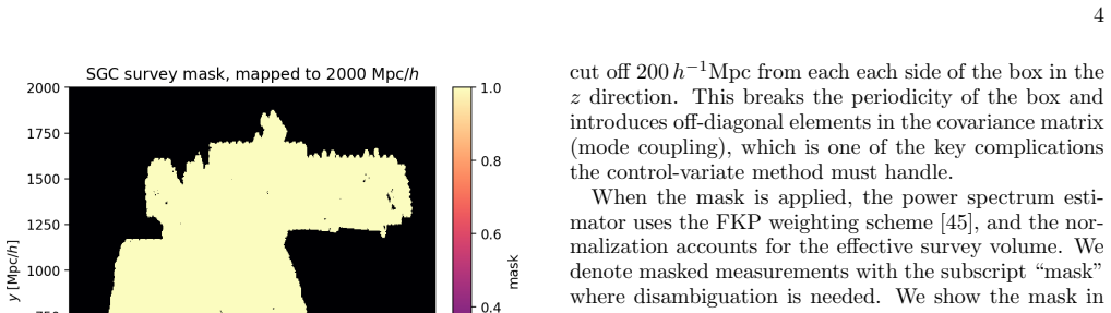
Survey mask To test the method in a realistic setting, we apply a survey window function modeled on the DESI South Galactic Cap (SGC) geometry at redshiftz= 0.5. The mask is a binary angular selection function applied to the simulation box; regions outside the observed region in thexycross-section are zeroed, and we additionally cut off 200h −1Mpc from ea...
-
[5]
Setup and notation Let ˆP (s) ℓ (k) denote the power spectrum multipole mea- sured from thes-th lognormal realization, and let ˆQ(s) ℓ (k) denote the corresponding measurement from the paired Zeldovich realization (same initial conditions). We orga- nize these into data vectorsd (s) andc (s) by concatenat- ing all (k, ℓ) bins: d(s) i = ˆP (s) ℓi (ki), c (...
-
[6]
They arenotmatrices acting on the data vector, but rather scalar coefficients for each element of the covariance ma- trix
Control variate estimator In our notation,β ij andρ ij are defined element-by- element in the (k, ℓ) space of the covariance matrix. They arenotmatrices acting on the data vector, but rather scalar coefficients for each element of the covariance ma- trix. We could thus denote the elements by a single index, e.g.,α≡ij, but we opt to use the standard double...
-
[7]
Xij = ˆΣaa ij , C ij = ˆΣbb ij ,(19) where notationais used to refer to the lognormal mocks, bto the Zeldovich approximation mocks
Setup The target and control quantities entering the control- variate estimator are elements of sample covariance ma- trices estimated fromN sim paired simulations. Xij = ˆΣaa ij , C ij = ˆΣbb ij ,(19) where notationais used to refer to the lognormal mocks, bto the Zeldovich approximation mocks. The covariance is estimated via ˆΣab ij = 1 Nsim −1 NsimX s=...
-
[8]
Covariance of the sample covariance matrix Under the Gaussian approximation, the fields are fully characterised by their two-point functions, and the co- variance of two-point estimators follows from the Isserlis– Wick theorem. For Gaussian fields, the binned power spectrum estimator satisfies Cov ˆP a(ki), ˆP b(kj) ≃ 2 [Pab(ki)]2 Nk,i δij ,(22) whereN k,...
-
[9]
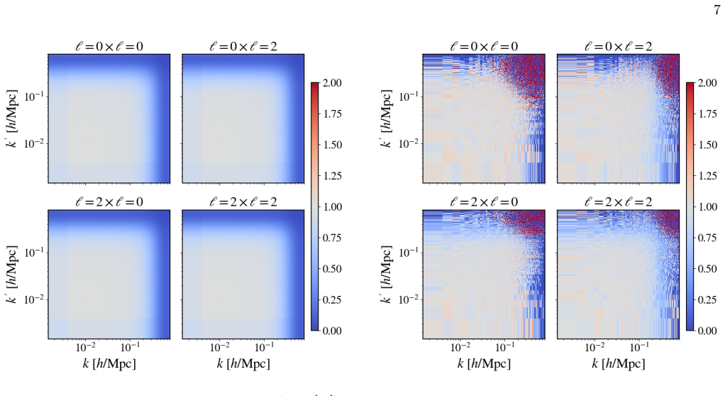
Analytic expressions forβandρ Taking the ratio of Eqs. (27) and (28), the (N sim −1) andN k factors cancel exactly, giving the main result: βij = Cov[Xij, C ij] Var[Cij] = [P ab(ki)]2 [P ab(kj)]2 [P bb(ki)]2 [P bb(kj)]2 .(30) Defining α(k)≡ [P ab(k)]2 [P bb(k)]2 ,(31) we write this as βij ≡α(k i)α(k j) (32) The correlation coefficient betweenX ij andC ij ...
-
[10]
projection ef- fects
Extension to multipoles The disconnected derivation above for the monopole relies only on the Gaussian covariance of the underlying bandpower estimators and on the fact that, in theµ- binning used there, differentµ-bins can be treated as ap- proximately independent. For redshift-space multipoles one can proceed analogously, but the crucial difference is t...
2000
-
[11]
The Zeldovich approximation provides an ex- tremely effective control variate: it is cheap to gen- erate and highly accurate on the same large scales where covariance estimation is most numerically challenging
-
[12]
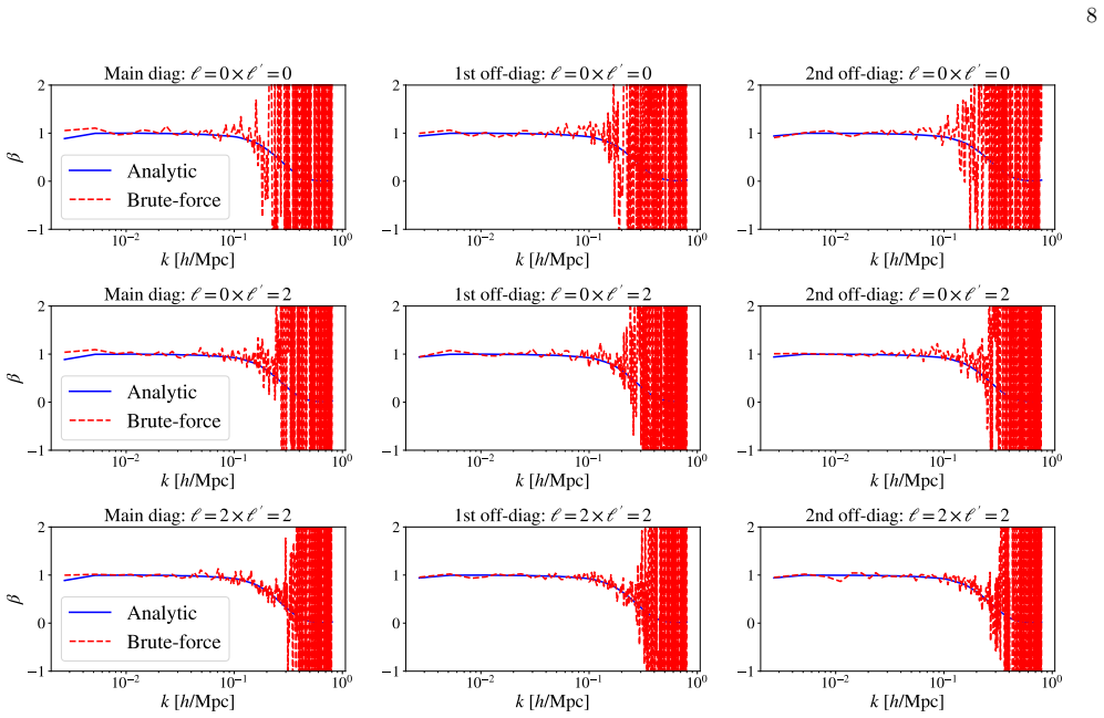
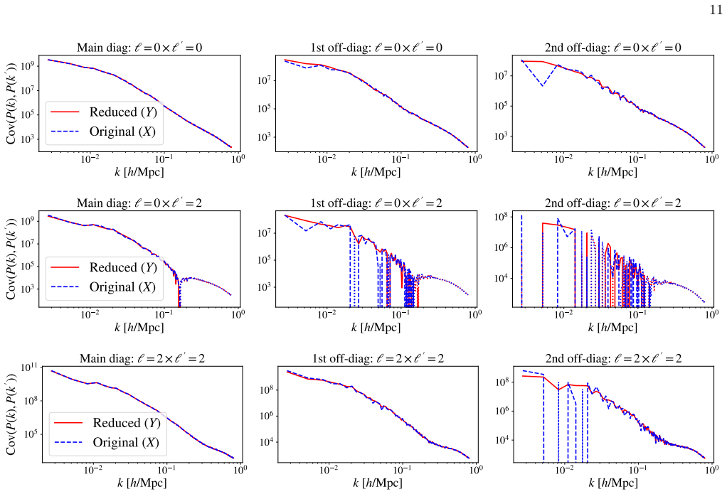
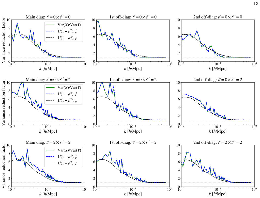
We derive an analytic expression for the opti- mal control-variate coefficientβ(k, ℓ;k ′, ℓ′), which is smooth and inexpensive; brute-force validation shows excellent agreement with the analytic pre- diction
-
[13]
We validate this dependence against brute-force computations (with a small systematic underpre- diction visible in one figure)
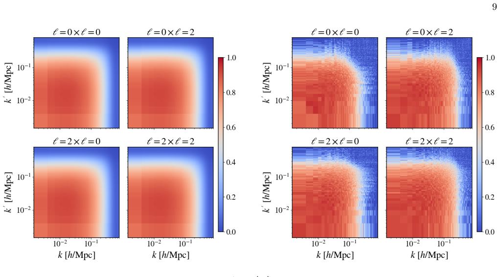
We derive an analytic expression forρ(k, ℓ;k ′, ℓ′), which depends only on the cross-correlation be- tween the target field and the Zeldovich control field; in the monopole caseρ(k, k ′) =r 2(k)r2(k′). We validate this dependence against brute-force computations (with a small systematic underpre- diction visible in one figure)
-
[14]
Despite the covariance involving products of fields, the performance penalty relative to power- spectrum control variates is modest: becauseρfac- torizes asr 2(ki)r2(kj), the resulting covariance per- formance is only about a factor of two worse than the naiver 2 expectation
-
[15]
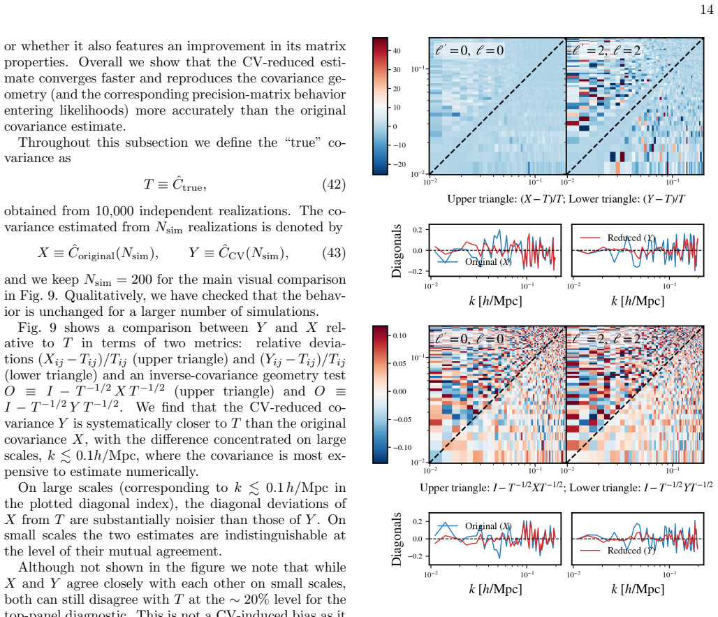
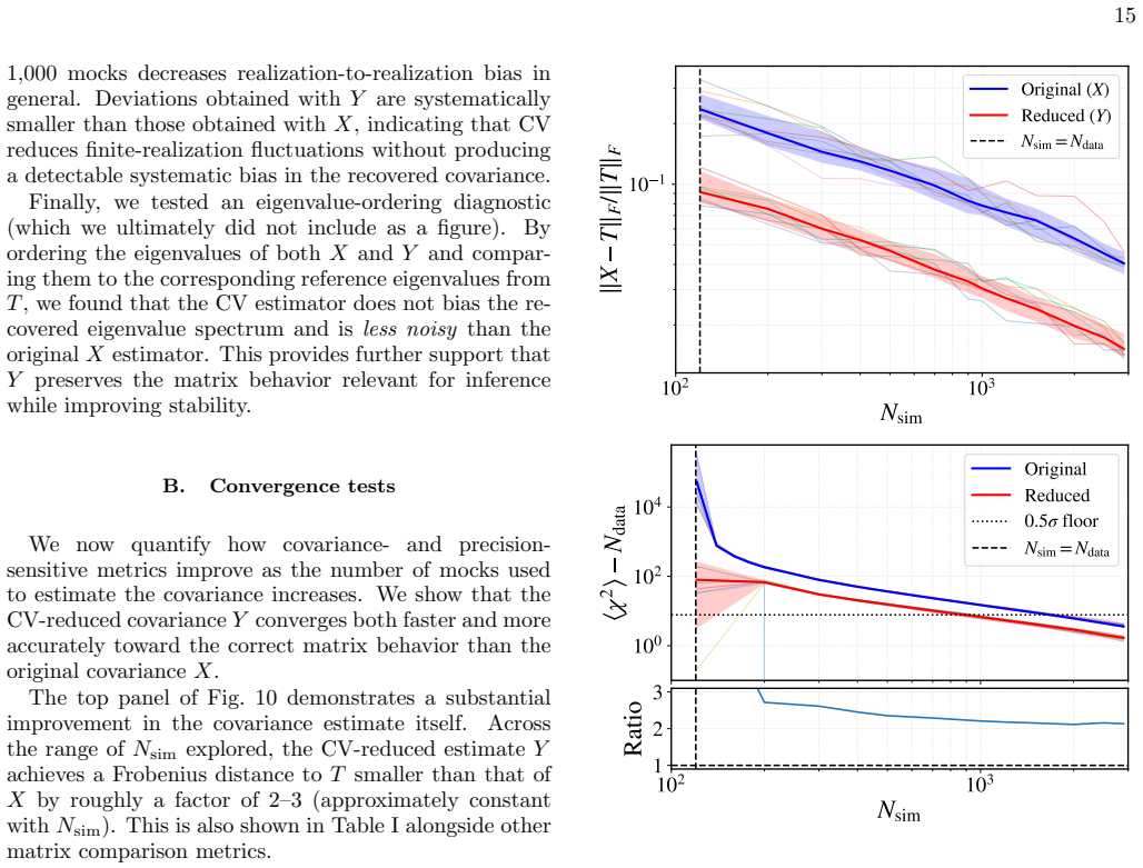
For DESI-like masked redshift-space lognormal mocks, the CV-reduced covariance achieves an O(10) variance-reduction gain on the largest scales, corresponding to an effective∼10 increase in the number of simulations needed for comparable co- variance accuracy
-
[16]
Looking ahead, several extensions are natural
Across a suite of covariance and precision-matrix- sensitive metrics, the CV-reduced estimate is con- sistently closer to the reference “truth” (by about a factor of∼3) and converges faster; whenN sim is close toN data, CV behaves like a shrinkage estima- tor and prevents the onset of ill-conditioning. Looking ahead, several extensions are natural. First,...
-
[17]
The Effect of Covariance Estimator Error on Cosmological Parameter Constraints
S. Dodelson and M. D. Schneider, Phys. Rev. D88, 063537 (2013), 1304.2593
work page internal anchor Pith review Pith/arXiv arXiv 2013
-
[18]
J. Hartlap, P. Simon, and P. Schneider, A&A464, 399 18 (2007), astro-ph/0608064
work page internal anchor Pith review Pith/arXiv arXiv 2007
-
[19]
Putting the Precision in Precision Cosmology: How accurate should your data covariance matrix be?
A. Taylor, B. Joachimi, and T. Kitching, MNRAS432, 1928 (2013), 1212.4359
work page internal anchor Pith review Pith/arXiv arXiv 1928
-
[20]
W. J. Percival, A. J. Ross, A. G. S´ anchez, L. Samushia, A. Burden, R. Crittenden, A. J. Cuesta, M. V. Magana, M. Manera, F. Beutler, et al., MNRAS439, 2531 (2014), 1312.4841
work page internal anchor Pith review Pith/arXiv arXiv 2014
-
[21]
Parameter inference with estimated covariance matrices
E. Sellentin and A. F. Heavens, MNRAS456, L132 (2016), 1511.05969
work page internal anchor Pith review Pith/arXiv arXiv 2016
-
[22]
The DESI Experiment Part I: Science,Targeting, and Survey Design
DESI Collaboration, A. Aghamousa, J. Aguilar, S. Ahlen, S. Alam, L. E. Allen, C. Allende Prieto, J. Annis, S. Bailey, C. Balland, et al., arXiv e-prints arXiv:1611.00036 (2016), 1611.00036
work page internal anchor Pith review Pith/arXiv arXiv 2016
-
[23]
Euclid Collaboration, Y. Mellier, Abdurro’uf, J. A. Acevedo Barroso, A. Ach´ ucarro, J. Adamek, R. Adam, G. E. Addison, N. Aghanim, M. Aguena, et al., A&A 697, A1 (2025), 2405.13491
-
[24]
Cosmology with the SPHEREX All-Sky Spectral Survey
O. Dor´ e, J. Bock, M. Ashby, P. Capak, A. Cooray, R. de Putter, T. Eifler, N. Flagey, Y. Gong, S. Habib, et al., arXiv e-prints arXiv:1412.4872 (2014), 1412.4872
work page internal anchor Pith review Pith/arXiv arXiv 2014
-
[25]
M. Takada, R. S. Ellis, M. Chiba, J. E. Greene, H. Ai- hara, N. Arimoto, K. Bundy, J. Cohen, O. Dor´ e, G. Graves, et al., PASJ66, R1 (2014), 1206.0737
work page internal anchor Pith review Pith/arXiv arXiv 2014
-
[26]
LSST Science Collaboration, P. A. Abell, J. Allison, S. F. Anderson, J. R. Andrew, J. R. P. Angel, L. Armus, D. Ar- nett, S. J. Asztalos, T. S. Axelrod, et al., arXiv e-prints arXiv:0912.0201 (2009), 0912.0201
work page internal anchor Pith review Pith/arXiv arXiv 2009
-
[27]
Power Spectrum Correlations Induced by Non-Linear Clustering
R. Scoccimarro, M. Zaldarriaga, and L. Hui, ApJ527, 1 (1999), astro-ph/9901099
work page internal anchor Pith review Pith/arXiv arXiv 1999
-
[28]
The Growth of Correlations in the Matter Power Spectrum
A. Meiksin and M. White, MNRAS308, 1179 (1999), astro-ph/9812129
work page internal anchor Pith review Pith/arXiv arXiv 1999
-
[29]
Response Approach to the Matter Power Spectrum Covariance
A. Barreira and F. Schmidt, J. Cosmology Astropart. Phys.2017, 051 (2017), 1705.01092
work page internal anchor Pith review Pith/arXiv arXiv 2017
-
[30]
D. Wadekar and R. Scoccimarro, Phys. Rev. D102, 123517 (2020), 1910.02914
- [31]
-
[32]
A. Cooray and R. Sheth, Phys. Rep.372, 1 (2002), astro- ph/0206508
-
[33]
Covariance of the galaxy angular power spectrum with the halo model
F. Lacasa, A&A615, A1 (2018), 1711.07372
work page internal anchor Pith review Pith/arXiv arXiv 2018
-
[34]
Simulations of Baryon Acoustic Oscillations II: Covariance matrix of the matter power spectrum
R. Takahashi, N. Yoshida, M. Takada, T. Matsubara, N. Sugiyama, I. Kayo, A. J. Nishizawa, T. Nishimichi, S. Saito, and A. Taruya, ApJ700, 479 (2009), 0902.0371
work page internal anchor Pith review Pith/arXiv arXiv 2009
-
[35]
L. Blot, M. Crocce, E. Sefusatti, M. Lippich, A. G. S´ anchez, M. Colavincenzo, P. Monaco, M. A. Alvarez, A. Agrawal, S. Avila, et al., MNRAS485, 2806 (2019), 1806.09497
work page internal anchor Pith review Pith/arXiv arXiv 2019
-
[36]
Comparing approximate methods for mock catalogues and covariance matrices I: correlation function
M. Lippich, A. G. S´ anchez, M. Colavincenzo, E. Se- fusatti, P. Monaco, L. Blot, M. Crocce, M. A. Alvarez, A. Agrawal, S. Avila, et al., MNRAS482, 1786 (2019), 1806.09477
work page internal anchor Pith review Pith/arXiv arXiv 2019
-
[37]
P. Norberg, C. M. Baugh, E. Gazta˜ naga, and D. J. Cro- ton, MNRAS396, 19 (2009), 0810.1885
work page internal anchor Pith review Pith/arXiv arXiv 2009
- [38]
-
[39]
A. C. Pope and I. Szapudi, MNRAS389, 766 (2008), 0711.2509
work page internal anchor Pith review Pith/arXiv arXiv 2008
-
[40]
D. J. Paz and A. G. S´ anchez, MNRAS454, 4326 (2015), 1508.03162
work page internal anchor Pith review Pith/arXiv arXiv 2015
-
[41]
Estimating sparse precision matrices
N. Padmanabhan, M. White, H. H. Zhou, and R. O’Connell, MNRAS460, 1567 (2016), 1512.01241
work page internal anchor Pith review Pith/arXiv arXiv 2016
-
[42]
Non-linear shrinkage estimation of large-scale structure covariance
B. Joachimi, MNRAS466, L83 (2017), 1612.00752
work page internal anchor Pith review Pith/arXiv arXiv 2017
-
[43]
O. Friedrich and T. Eifler, MNRAS473, 4150 (2018), 1703.07786
work page internal anchor Pith review Pith/arXiv arXiv 2018
-
[44]
D. Wadekar, M. M. Ivanov, and R. Scoccimarro, Phys. Rev. D102, 123521 (2020), 2009.00622
-
[45]
S. M. Ross,Simulation(Academic Press, Inc., USA, 2002), 3rd ed., ISBN 0125980531
2002
-
[46]
N. Chartier, B. Wandelt, Y. Akrami, and F. Villaescusa- Navarro, MNRAS503, 1897 (2021), 2009.08970
-
[47]
N. Chartier and B. D. Wandelt, MNRAS509, 2220 (2022), 2106.11718
-
[48]
N. Chartier and B. D. Wandelt, MNRAS515, 1296 (2022), 2204.03070
-
[49]
N. Kokron, S.-F. Chen, M. White, J. DeRose, and M. Maus, J. Cosmology Astropart. Phys.2022, 059 (2022), 2205.15327
-
[50]
J. DeRose, S.-F. Chen, N. Kokron, and M. White, J. Cos- mology Astropart. Phys.2023, 008 (2023), 2210.14239
-
[51]
Control variates from Eulerian and Lagrangian perturbation theory: Application to the bispectrum
N. Kokron and S.-F. Chen, arXiv e-prints arXiv:2510.07375 (2025), 2510.07375
work page internal anchor Pith review Pith/arXiv arXiv 2025
-
[52]
B. Hadzhiyska, M. J. White, X. Chen, L. H. Garri- son, J. DeRose, N. Padmanabhan, C. Garcia-Quintero, J. Mena-Fern´ andez, S.-F. Chen, H.-J. Seo, et al., The Open Journal of Astrophysics6, 38 (2023), 2308.12343
-
[53]
Simulation budgeting for hybrid effective field theories
A. Bartlett, J. DeRose, and M. White, J. Cosmology As- tropart. Phys.2026, 078 (2026), 2510.13962
work page internal anchor Pith review Pith/arXiv arXiv 2026
-
[54]
D. Blas, J. Lesgourgues, and T. Tram, J. Cosmology As- tropart. Phys.2011, 034 (2011), 1104.2933
work page internal anchor Pith review Pith/arXiv arXiv 2011
-
[55]
Y. B. Zel’dovich, A&A5, 84 (1970)
1970
-
[56]
K. Yamamoto, ApJ595, 577 (2003), astro-ph/0208139
work page internal anchor Pith review Pith/arXiv arXiv 2003
-
[57]
Coles and B
P. Coles and B. Jones, MNRAS248, 1 (1991)
1991
- [58]
- [59]
-
[60]
R. W. Hockney and J. W. Eastwood,Computer Simula- tion Using Particles(1981)
1981
-
[61]
H. A. Feldman, N. Kaiser, and J. A. Peacock, ApJ426, 23 (1994), astro-ph/9304022
work page internal anchor Pith review Pith/arXiv arXiv 1994
-
[62]
Bhatia,Positive Definite Matrices, Princeton Series in Applied Mathematics (Princeton University Press, 2009), ISBN 9781400827787, URLhttps://books
R. Bhatia,Positive Definite Matrices, Princeton Series in Applied Mathematics (Princeton University Press, 2009), ISBN 9781400827787, URLhttps://books. google.com/books?id=-KIFglY18nYC
2009
-
[63]
R. A. Horn and C. R. Johnson,Matrix Analysis(Cam- bridge University Press, Cambridge, UK, 2012), 2nd ed., ISBN 9780521839402
2012
discussion (0)
Sign in with ORCID, Apple, or X to comment. Anyone can read and Pith papers without signing in.