Total, quantum, and classical measures of anticoherence for mixed spin states
Pith reviewed 2026-06-29 07:17 UTC · model grok-4.3
The pith
Mixed spin states decompose their anticoherence into total, quantum, and classical contributions via an axiomatic framework on the symmetric qubit embedding.
A machine-rendered reading of the paper's core claim, the machinery that carries it, and where it could break.
Core claim
Anticoherent spin states possess isotropic low-order spin moments. For mixed states this isotropy can arise either from quantum correlations or from classical mixing. The framework defines total t-anticoherence to be non-decreasing under SU(2)-covariant channels. Quantum t-anticoherence is introduced as a resource monotone relative to a chosen total measure, required to coincide with it on all pure states; their difference is the classical contribution. Total measures are built from reduced-state purity, Hilbert-Schmidt distance, and cumulative multipoles; quantum counterparts use convex-roof extensions of pure-state functionals tied to bipartite entanglement in the symmetric sector. Example
What carries the argument
The symmetric qubit embedding, which maps spin-j states to symmetric multi-qubit states so that t-anticoherence measures can be defined from reduced-state properties and bipartite entanglement in that sector.
If this is right
- Total measures can be constructed from reduced-state purity, Hilbert-Schmidt distance, and cumulative multipoles.
- Quantum measures are obtained via convex-roof extensions of pure-state functionals tied to symmetric-sector entanglement.
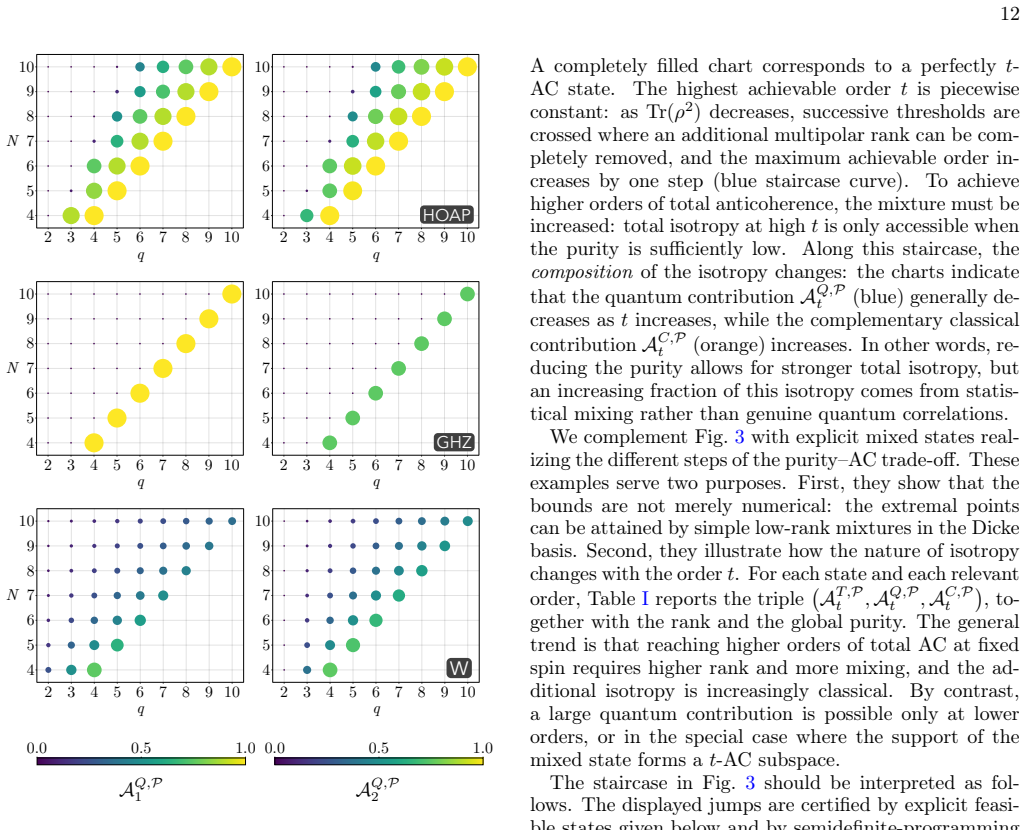
- States exist that achieve maximal quantum anticoherence while supported on anticoherent subspaces.
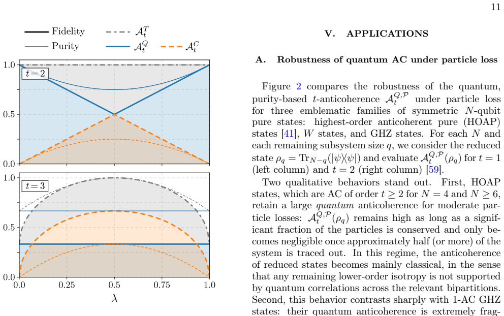
- Robustness of the measures under particle loss differs by state type.
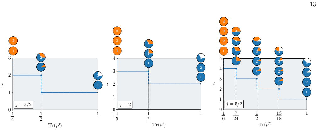
- A trade-off exists between state purity and the highest achievable anticoherence order.
Where Pith is reading between the lines
- The total-versus-quantum split may let metrology protocols be tuned to suppress the classical part while preserving the quantum resource.
- The same convex-roof technique could be transferred to other resource theories that already separate quantum and classical contributions.
- Explicit formulas for low-j cases could be used to test whether the measures remain useful when the symmetric embedding is relaxed.
Load-bearing premise
A quantum t-anticoherence measure can be consistently defined via convex-roof extensions of pure-state functionals that coincide exactly with the total measure on every pure state.
What would settle it
A concrete mixed state for which the constructed quantum measure either fails to coincide with the total measure on its pure-state support or decreases under an SU(2)-covariant channel.
Figures
read the original abstract
Anticoherent spin states have isotropic low-order spin moments and are relevant to direction-independent metrology and quantum reference-frame alignment. In contrast to pure states, for mixed states such isotropy may originate either from genuine quantum correlations or from classical statistical mixing. We introduce an axiomatic framework for mixed-state $t$-anticoherence based on the symmetric qubit embedding. We distinguish total $t$-anticoherence, non-decreasing under SU(2)-covariant channels, from quantum $t$-anticoherence, defined as a resource monotone relative to a chosen total measure and constrained to coincide with it on pure states. This yields a classical contribution as their difference. We construct total measures based on reduced-state purity, Hilbert-Schmidt distance, and cumulative multipoles, and we discuss fidelity-based total candidates. We construct quantum counterparts via convex-roof extensions of pure-state functionals tied to bipartite entanglement in the symmetric sector. We provide explicit mixed-state examples, identify states with maximal quantum anticoherence supported on anticoherent subspaces, study robustness under particle loss for different types of states, and characterize the trade-off between purity and the maximal achievable anticoherence order.
Editorial analysis
A structured set of objections, weighed in public.
Referee Report
Summary. The manuscript introduces an axiomatic framework for t-anticoherence of mixed spin states via the symmetric qubit embedding. Total t-anticoherence is defined to be non-decreasing under SU(2)-covariant channels; quantum t-anticoherence is a resource monotone relative to a chosen total measure that is required to coincide exactly with it on all pure states; the classical contribution is their difference. Total measures are constructed from reduced-state purity, Hilbert-Schmidt distance to the maximally mixed state, and cumulative multipole moments (with fidelity-based candidates also discussed). Quantum counterparts are obtained via convex-roof extensions of pure-state functionals tied to bipartite entanglement in the symmetric sector. The work supplies explicit mixed-state examples, identifies states with maximal quantum anticoherence supported on anticoherent subspaces, studies robustness under particle loss, and characterizes the purity-anticoherence trade-off.
Significance. If the claimed monotonicity and coincidence properties hold, the framework supplies a principled separation of quantum and classical origins of isotropy in spin moments, which is relevant to direction-independent metrology and quantum reference-frame tasks. Credit is due for grounding the constructions in standard tools (convex-roof extensions, entanglement monotones) and for supplying explicit examples together with robustness and trade-off analyses; these elements make the measures immediately usable for further study.
Simulated Author's Rebuttal
We thank the referee for their positive summary, significance assessment, and recommendation to accept the manuscript. No major comments were raised, so we have no revisions or responses to provide on specific points.
Circularity Check
No significant circularity
full rationale
The paper introduces an axiomatic framework distinguishing total t-anticoherence (non-decreasing under SU(2)-covariant channels) from quantum t-anticoherence (resource monotone coinciding on pure states, obtained via convex-roof of pure-state functionals tied to symmetric-sector entanglement). Total measures are constructed from standard quantities (reduced-state purity, Hilbert-Schmidt distance to maximally mixed state, cumulative multipole moments) and fidelity candidates. Quantum versions follow the canonical convex-roof procedure. These steps rely on established concepts in quantum information (purity, monotones, convex-roof extensions) without reducing any central claim to a fitted parameter renamed as prediction, a self-definitional loop, or a load-bearing self-citation chain. The derivation chain is self-contained against external benchmarks and does not exhibit any of the enumerated circularity patterns.
Axiom & Free-Parameter Ledger
axioms (2)
- domain assumption Symmetric qubit embedding provides the appropriate representation for defining t-anticoherence of mixed spin states
- domain assumption Quantum t-anticoherence must coincide with total t-anticoherence on all pure states
Reference graph
Works this paper leans on
-
[1]
Pairwise orthogonal partial transposed projectors By definition, the negativity satisfies N CR t (ρ)≥ N t(ρ).(82) A sufficient condition for saturation is the following: con- sider a decomposition of the stateρ= P i pi |ψi⟩⟨ψi|. If the images of the partially transposed projectors (|ψi⟩⟨ψi|)TA are pairwise orthogonal subspaces7, then the negativity is add...
-
[2]
no- loss
Fort= 1, both measures giveA T 1 =A Q 1 = 1andA C 1 = 0(data not shown). an AC subspace (see Appendix F in Ref. [29]). However, they are not the only cases. Another nontrivial example that does not arise from an AC subspace is given by two spin-5/2states: |ψ1⟩= 1√ 6 | 5 2 ,− 5 2 ⟩+ q 5 6 | 5 2 , 3 2 ⟩, |ψ2⟩=− q 5 6 | 5 2 ,− 3 2 ⟩+ 1√ 6 | 5 2 , 5 2 ⟩. (85)...
-
[3]
1 Proof.First,Tr(ρ 2 t ) = 1/(t+ 1)if and only ifρ t is maxi- mally mixed, which gives (T1)
Proof of Prop. 1 Proof.First,Tr(ρ 2 t ) = 1/(t+ 1)if and only ifρ t is maxi- mally mixed, which gives (T1). Let us now prove (T2). Ifρis a pure coherent state, then every reduced stateρ t is pure, soTr(ρ 2 t ) = 1and henceA T,P t (ρ) = 0. Conversely, ifA T,P t (ρ) = 0, then Tr(ρ2 t ) = 1, soρ t is pure. Sinceρ t is obtained by tracing out part of the symm...
-
[4]
2 Proof.Axioms (T1)–(T3) follow from the general distance-based construction
Proof of Prop. 2 Proof.Axioms (T1)–(T3) follow from the general distance-based construction. We now prove (T4) as in Prop. 1. Using the notation (A7) together with the ex- 16 pansion ofρ t in Eq. (6), we have ∥(Φ(ρ))t −ρ (t) 0 ∥2 2 = tX L=1 LX M=−L c2 N,t,L|fL|2 |ρLM |2 ≤ tX L=1 LX M=−L c2 N,t,L|ρLM |2 =∥ρ t −ρ (t) 0 ∥2 2, (A10) because|f L| ≤1for allL. H...
-
[5]
Proof of Prop. 3 Proof.From the Schmidt decomposition, it can be seen that the reduced state of|ψ⟩onAis given by ρA = dAX i=1 α2 i |ϕ(i) A ⟩ ⟨ϕ(i) A |,(A12) So, the eigenvaluesλ i ofρ A are related to the Schmidt coefficientsα i, that is,λ i =α 2 i. For pure statesρ= |ψ⟩⟨ψ|, the fidelity betweenρA and the MMS verifies F(ρ A, ρ0) = 1 dA (Tr√ρA)2 = 1 dA dAX...
-
[6]
4 Proof.Pure-state consistency (Q2) andSU(2)invariance (Q3)areimmediatefromthedefinitionandtherotational covariance of the reduced state
Proof of Prop. 4 Proof.Pure-state consistency (Q2) andSU(2)invariance (Q3)areimmediatefromthedefinitionandtherotational covariance of the reduced state. Convexity (Q4) follows directly from the convex-roof construction. Axiom (Q5) follows from Theorem 2 since the functionf(ρ) = 1− Tr(ρ2)is concave and invariant under unitaries due to the properties of the...
-
[7]
Proof of Prop. 5 Proof.For pure states|ψ⟩, the reduced density matrices across the bipartitionst|N−tand(N−t)|thave iden- tical nonzero spectra, which impliesTr(ρ2 t ) = Tr(ρ 2 N−t) and therefore AP t (|ψ⟩) =c t AP N−t(|ψ⟩), c t = (t+ 1)(N−t) t(N+ 1−t) .(A16) Letρ= P i pi|ψi⟩⟨ψi|be an arbitrary pure-state decom- position. Using the above relation term by t...
-
[8]
6 Proof.Axioms (Q2) and (Q4) follow directly from the convex-roof construction, while axiom (Q3) follows from theSU(2)invariance of the pure-state functional
Proof of Prop. 6 Proof.Axioms (Q2) and (Q4) follow directly from the convex-roof construction, while axiom (Q3) follows from theSU(2)invariance of the pure-state functional. Ax- iom (Q5) follows by assumption, sinceAd t (|ψ⟩)is an en- tanglement monotone across the bipartitiont|N−tand convex roofs of pure-state entanglement monotones are LOCC monotones. A...
-
[9]
7 Proof.We first recall the definition of the total fidelity- based measure: AT,F t (ρ) = (Tr(√ρt))2 −1 t = (t+ 1)F(ρ t, ρ(t) 0 )−1 t
Proof of Prop. 7 Proof.We first recall the definition of the total fidelity- based measure: AT,F t (ρ) = (Tr(√ρt))2 −1 t = (t+ 1)F(ρ t, ρ(t) 0 )−1 t . (A19) 17 As discussed in Sec. IIIA3, this quantity satisfies axioms (T1)–(T3). Indeed, (T1) follows fromF(ρ t, ρ(t) 0 ) = 1 iffρ t =ρ (t) 0 , while (T2) follows from the fact that F(ρ t, ρ(t) 0 ) = 1/(t+ 1)...
-
[10]
8 Proof.We first show thatA T,cm t (ρ)is indeed a function taking values in[0,1], which is equivalent to proving that 0≤C ≤t(ρ)≤C ≤t(ρcoh)
Proof of Prop. 8 Proof.We first show thatA T,cm t (ρ)is indeed a function taking values in[0,1], which is equivalent to proving that 0≤C ≤t(ρ)≤C ≤t(ρcoh). Since it is a sum of positive quantities, it is immediate to verify thatC ≤t(ρ)≥0. The upper bound is proved in the following lemma: Lemma 2.For every spin-jdensity matrixρand every t= 1, . . . ,2j−1, C...
-
[11]
9 Proof.Fort= 1,C ≤1(ρ)is affine in the one-body re- duced purityr 1 = Tr(ρ 2 1)(equivalently, in|⟨J⟩| 2) by the standard purity–multipole relations for symmetric states
Proof of Prop. 9 Proof.Fort= 1,C ≤1(ρ)is affine in the one-body re- duced purityr 1 = Tr(ρ 2 1)(equivalently, in|⟨J⟩| 2) by the standard purity–multipole relations for symmetric states. Therefore, after normalization to[0,1]with co- herent states mapped to0and1-AC pure states to1, the pure-state functionalsA T,cm 1 (|ψ⟩)andA P 1 (|ψ⟩)coincide. Taking conv...
-
[12]
Zimba, Electronic Journal of Theoretical Physics3, 143 (2006)
J. Zimba, Electronic Journal of Theoretical Physics3, 143 (2006)
2006
-
[13]
Rudziński, A
M. Rudziński, A. Burchardt, and K. Życzkowski, Quan- tum8, 1234 (2024)
2024
-
[14]
Björk, A
G. Björk, A. B. Klimov, P. de la Hoz, M. Grassl, G. Leuchs, and L. L. Sánchez-Soto, Phys. Rev. A92, 031801(R) (2015)
2015
-
[15]
Crann, R
J. Crann, R. Pereira, and D. W. Kribs, J. Phys. A: Math. Theor.43, 255307 (2010)
2010
-
[16]
Baguette, F
D. Baguette, F. Damanet, O. Giraud, and J. Martin, Phys. Rev. A92, 052333 (2015)
2015
-
[17]
Serrano-Ensástiga and D
E. Serrano-Ensástiga and D. Braun, Phys. Rev. A101, 022332 (2020)
2020
-
[18]
Baguette, T
D. Baguette, T. Bastin, and J. Martin, Phys. Rev. A90, 032314 (2014)
2014
-
[19]
Kolenderski and R
P. Kolenderski and R. Demkowicz-Dobrzanski, Phys. Rev. A78, 052333 (2008)
2008
-
[20]
Chryssomalakos and H
C. Chryssomalakos and H. Hernández-Coronado, Phys. Rev. A95, 052125 (2017)
2017
-
[21]
A. Z. Goldberg and D. F. V. James, Phys. Rev. A98, 032113 (2018)
2018
-
[22]
Martin, S
J. Martin, S. Weigert, and O. Giraud, Quantum4, 285 (2020)
2020
-
[23]
Ferretti, Y
H. Ferretti, Y. B. Yilmaz, K. Bonsma-Fisher, A. Z. Gold- berg, N. Lupu-Gladstein, A. O. T. Pang, L. A. Rozema, and A. M. Steinberg, Optica Quantum2, 91 (2024)
2024
-
[24]
J. M. Robbins and M. V. Berry, Journal of Physics A: Mathematical and General27, L435 (1994)
1994
-
[25]
Aguilar, C
P. Aguilar, C. Chryssomalakos, E. Guzmán-González, L. Hanotel, and E. Serrano-Ensástiga, Journal of Physics A: Mathematical and Theoretical53, 065301 (2020)
2020
-
[26]
Chryssomalakos, L
C. Chryssomalakos, L. Hanotel, E. Guzmán-González, and E. Serrano-Ensástiga, Mod. Phys. Lett. A37, 2250184 (2022)
2022
-
[27]
Hervas, A.Z.Goldberg, A.S.Sanz, Z.Hradil, J
J.R. Hervas, A.Z.Goldberg, A.S.Sanz, Z.Hradil, J. Ře- háček, and L. L. Sánchez-Soto, Phys. Rev. Lett.134, 010804 (2025)
2025
-
[28]
Chiew and M
S.-H. Chiew and M. Gessner, Phys. Rev. Res.4, 013076 (2022)
2022
-
[29]
Massar and S
S. Massar and S. Popescu, Phys. Rev. Lett.74, 1259 (1995)
1995
-
[30]
Gisin and S
N. Gisin and S. Popescu, Phys. Rev. Lett.83, 432 (1999)
1999
-
[31]
Peres and P
A. Peres and P. F. Scudo, Phys. Rev. Lett.86, 4160 (2001)
2001
-
[32]
Peres and P
A. Peres and P. F. Scudo, Phys. Rev. Lett.87, 167901 (2001)
2001
-
[33]
Peres and P
A. Peres and P. Scudo, Journal of Modern Optics49, 1235 (2002)
2002
-
[34]
D. Collins and S. Popescu, arXiv preprint quant- ph/0401096 (2004), arXiv:quant-ph/0401096
-
[36]
S. D. Bartlett, T. Rudolph, and R. W. Spekkens, Rev. Mod. Phys.79, 555 (2007)
2007
-
[37]
Gour and R
G. Gour and R. W. Spekkens, New J. Phys.10, 033023 (2008)
2008
-
[38]
G. Gour, I. Marvian, and R. W. Spekkens, Phys. Rev. A 80, 012307 (2009)
2009
-
[39]
Chitambar and G
E. Chitambar and G. Gour, Rev. Mod. Phys.91, 025001 (2019)
2019
-
[40]
Serrano-Ensástiga, C
E. Serrano-Ensástiga, C. Chryssomalakos, and J. Martin, Phys. Rev. A111, 022435 (2025)
2025
-
[41]
Bouchard, P
F. Bouchard, P. de la Hoz, G. Björk, R. W. Boyd, M.Grassl, Z.Hradil, E.Karimi, A.B.Klimov, G.Leuchs, J. Řeháček, and L. L. Sánchez-Soto, Optica4, 1429 (2017)
2017
-
[42]
Denis, C
J. Denis, C. Read, and J. Martin, SciPost Phys. Core9, 001 (2026). 19
2026
-
[43]
A. Z. Goldberg, J. R. Hervas, A. S. Sanz, A. B. Klimov, J. Řeháček, Z. Hradil, M. Hiekkamäki, M. Eriksson, R. Fickler, G. Leuchs, and L. L. Sánchez-Soto, Quantum Science and Technology10, 015053 (2024)
2024
-
[44]
Butterfly Echo Protocol for Axis-Agnostic Heisenberg-Limited Metrology
J. Bringewatt, L. Zaporski, M. Radzihovsky, J. Albert, A. V. Gorshkov, V. Vuletic, and G. Bentsen, Butterfly echo protocol for axis-agnostic heisenberg-limited metrol- ogy (2026), arXiv:2602.23332 [quant-ph]
work page internal anchor Pith review Pith/arXiv arXiv 2026
-
[45]
Baguette and J
D. Baguette and J. Martin, Phys. Rev. A96, 032304 (2017)
2017
-
[46]
Majorana, Il Nuovo Cimento (1924-1942)9, 43 (1932)
E. Majorana, Il Nuovo Cimento (1924-1942)9, 43 (1932)
1924
-
[47]
Aulbach, D
M. Aulbach, D. Markham, and M. Murao, New J. Phys. 12, 073025 (2010)
2010
-
[48]
Aulbach, Int
M. Aulbach, Int. J. Quantum Inf.10, 1230004 (2012)
2012
-
[49]
de la Hoz, A
P. de la Hoz, A. B. Klimov, G. Björk, Y.-H. Kim, C. Müller, C. Marquardt, G. Leuchs, and L. L. Sánchez- Soto, Phys. Rev. A88, 063803 (2013)
2013
-
[50]
L. L. Sánchez-Soto, A. B. Klimov, P. de la Hoz, and G. Leuchs, J. Phys. B: At. Mol. Opt. Phys.46, 104011 (2013)
2013
-
[51]
D. A. Varshalovich, A. N. Moskalev, and V. K. Kher- sonskii,Quantum Theory of Angular Momentum(World Scientific, 1988)
1988
-
[52]
Denis and J
J. Denis and J. Martin, Phys. Rev. Res.4, 013178 (2022)
2022
-
[53]
Giraud, D
O. Giraud, D. Braun, D. Baguette, T. Bastin, and J. Martin, Phys. Rev. Lett.114, 080401 (2015)
2015
-
[54]
Marvian and R
I. Marvian and R. W. Spekkens, Nat. Commun.5, 3821 (2014)
2014
-
[55]
Marvian and R
I. Marvian and R. W. Spekkens, Phys. Rev. A90, 014102 (2014)
2014
-
[56]
A. S. Holevo, Remarks on the classical capacity of quan- tum channel (2002), arXiv:quant-ph/0212025
work page internal anchor Pith review Pith/arXiv arXiv 2002
-
[57]
Müller, Diffusive spin transport, inEntanglement and Decoherence: Foundations and Modern Trends, edited by A
C. Müller, Diffusive spin transport, inEntanglement and Decoherence: Foundations and Modern Trends, edited by A. Buchleitner, C. Viviescas, and M. Tiersch (Springer Berlin Heidelberg, Berlin, Heidelberg, 2009) pp. 277–314
2009
-
[58]
Rivas and A
Á. Rivas and A. Luis, Phys. Rev. A88, 052120 (2013)
2013
-
[59]
Chang, J
E. Chang, J. Kim, H. Kwak, H. H. Lee, and S.-G. Youn, Reviews in Mathematical Physics34, 2250021 (2022)
2022
-
[60]
Aschieri, B
T. Aschieri, B. Ruba, and J. P. Solovej, Communications in Mathematical Physics405, 298 (2024)
2024
-
[61]
Ichikawa, T
T. Ichikawa, T. Sasaki, I. Tsutsui, and N. Yonezawa, Physical Review A78, 052105 (2008)
2008
-
[62]
Vidal and R
G. Vidal and R. F. Werner, Phys. Rev. A65, 032314 (2002)
2002
-
[63]
S. Lee, D. P. Chi, S. D. Oh, and J. Kim, Phys. Rev. A 68, 062304 (2003)
2003
-
[64]
A. Z. Goldberg, A. B. Klimov, H. deGuise, G. Leuchs, G. S. Agarwal, and L. L. Sánchez-Soto, Optics Letters 47, 477 (2022)
2022
-
[65]
A. Z. Goldberg, P. de la Hoz, G. Björk, A. B. Klimov, M. Grassl, G. Leuchs, and L. L. Sánchez-Soto, Advances in Optics and Photonics13, 1 (2021)
2021
-
[66]
M. A. Nielsen, Phys. Rev. Lett.83, 436 (1999)
1999
-
[67]
Pereira and C
R. Pereira and C. Paul-Paddock, J. Math. Phys.58, 062107 (2017)
2017
-
[68]
J. A. Gross, Phys. Rev. Lett.127, 010504 (2021)
2021
-
[69]
S.Lim, J.Liu,andA.Ardavan,Phys.Rev.A108,062403 (2023)
2023
-
[70]
X. Zhu, C. Zhang, Z. An, and B. Zeng, npj Quantum Information11, 56 (2025)
2025
-
[71]
Kłobus, A
W. Kłobus, A. Burchardt, A. Kołodziejski, M. Pandit, T. Vértesi, K. Życzkowski, and W. Laskowski, Phys. Rev. A100, 032112 (2019)
2019
-
[72]
Vidal, Journal of Modern Optics47, 355 (2000)
G. Vidal, Journal of Modern Optics47, 355 (2000)
2000
-
[73]
Bourin and F
J.-C. Bourin and F. Hiai, International Journal of Math- ematics22, 1121 (2011)
2011
discussion (0)
Sign in with ORCID, Apple, or X to comment. Anyone can read and Pith papers without signing in.