Finite-key feasibility of geostationary quantum key distribution
Pith reviewed 2026-06-29 06:53 UTC · model grok-4.3
The pith
Geostationary satellite quantum key distribution achieves positive secret key rates with finite-key decoy-state BB84 protocols despite high loss and noise.
A machine-rendered reading of the paper's core claim, the machinery that carries it, and where it could break.
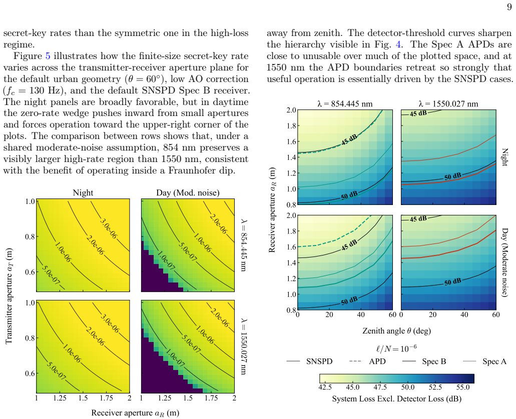
Core claim
Incorporating variable-length finite-key security and tight statistical bounds into the decoy-state BB84 protocol expands the positive-key regime for GEO downlink QKD, making it feasible under a physically realistic channel model that includes extreme loss, variable cloud cover, and background noise across environments and wavelengths.
What carries the argument
The physically realistic channel model that captures dominant loss and noise mechanisms, paired with finite-key security analysis applied to principal receiver architectures in the GEO downlink configuration.
If this is right
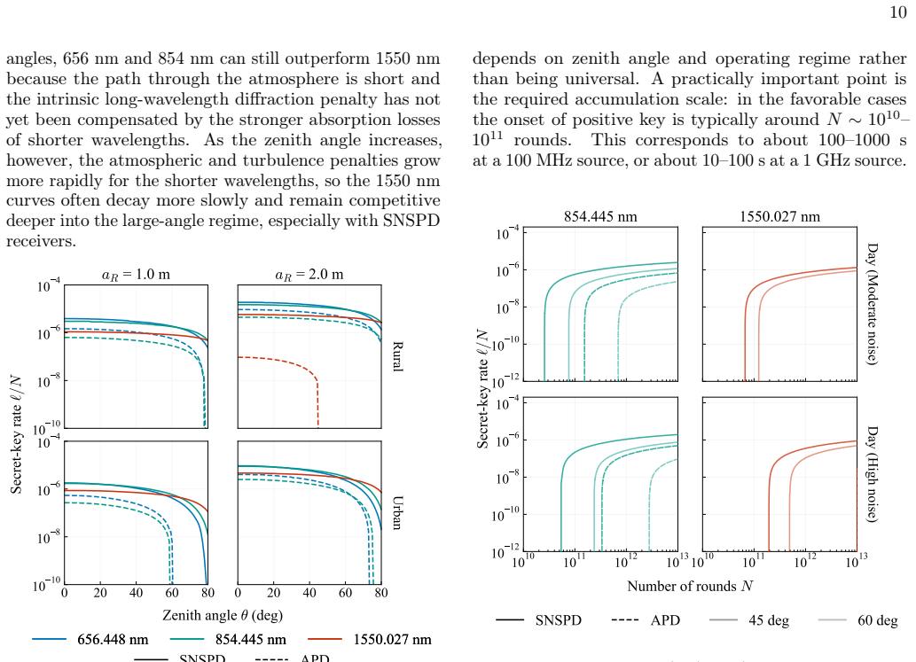
- Positive secret key rates become achievable in rural, urban, and coastal environments at visible Fraunhofer minima and telecom wavelengths.
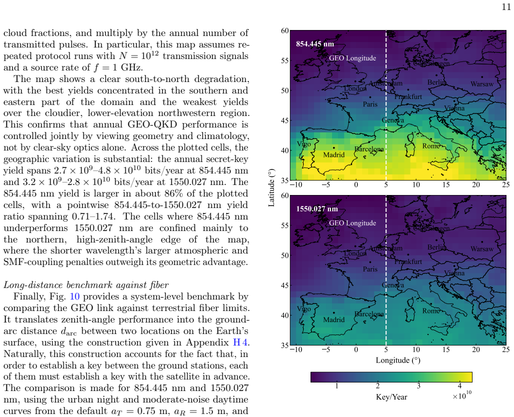
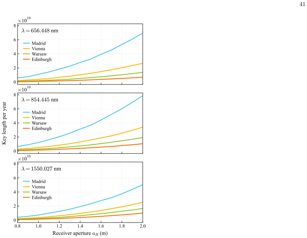
- Annual secret-key yields across Europe can be forecasted from historical cloud data.
- Systematic mapping of the parameter space identifies the key trade-offs and performance bottlenecks that govern feasibility.
- Practical operating thresholds and actionable design guidelines emerge for future GEO-QKD missions.
Where Pith is reading between the lines
- Confirmation would favor GEO platforms for continuous coverage rather than relying solely on low-Earth-orbit constellations.
- The thresholds could directly shape choices of wavelength, receiver design, and operational windows in mission planning.
- Sensitivity tests against unmodeled extremes such as prolonged cloud cover would strengthen or limit the forecasts.
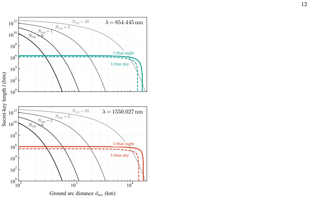
- Hybrid systems linking GEO downlinks to ground fiber networks could extend secure reach beyond single-satellite footprints.
Load-bearing premise
The channel model accurately captures the dominant loss and noise mechanisms including variable cloud cover and background noise levels across environments.
What would settle it
An actual GEO satellite QKD experiment that measures secret key rates falling below the calculated positive thresholds in the modeled rural, urban, or coastal scenarios would disprove the feasibility.
Figures
read the original abstract
Quantum key distribution (QKD) via geostationary Earth orbit (GEO) satellites offers a compelling route to continuous, continental-scale secure communications. However, operation in this regime entails extreme channel loss and significant background noise, particularly if daylight operation is desired. We present a comprehensive end-to-end feasibility study of a decoy-state BB84 protocol in a GEO downlink configuration, incorporating variable-length finite-key security and tight statistical bounds to expand the achievable positive-key regime. Our analysis encompasses the principal receiver architectures relevant to downlink QKD and employs a physically realistic channel model that captures the dominant loss and noise mechanisms. We evaluate performance across rural, urban, and coastal environments at multiple wavelengths, including visible Fraunhofer absorption minima and the telecom band. Using historical cloud data across Europe, we forecast the annual secret-key yield across the continent. Through a systematic exploration of the high-dimensional parameter space, we identify key trade-offs and performance bottlenecks that determine feasibility. These results establish practical operating thresholds and provide actionable design guidelines for future GEO-QKD missions.
Editorial analysis
A structured set of objections, weighed in public.
Referee Report
Summary. The manuscript conducts a comprehensive end-to-end feasibility study of decoy-state BB84 QKD in a GEO satellite downlink. It incorporates variable-length finite-key security analysis with tight statistical bounds, a physically realistic channel model for loss and noise (including variable cloud cover), and historical cloud data to forecast annual secret-key yields across Europe in rural, urban, and coastal settings at multiple wavelengths. The work systematically explores the high-dimensional parameter space to identify trade-offs, performance bottlenecks, and practical operating thresholds for future missions.
Significance. If the calculations are accurate, the results provide actionable design guidelines and operating thresholds for GEO-QKD systems under realistic conditions, including daylight operation. The combination of finite-key analysis with environmental forecasting using historical data is a strength that enhances the practical relevance of the feasibility claims.
minor comments (2)
- [Abstract] Abstract: the phrase 'variable-length finite-key security and tight statistical bounds' would benefit from a parenthetical reference to the specific bound family (e.g., 'using the variable-length analysis of Ref. X') to allow readers to locate the exact security proof immediately.
- The manuscript should explicitly state the range of free parameters explored (channel loss, background rates, finite-key block sizes) and whether any were tuned post hoc to achieve positive key rates; this would strengthen the independence of the reported thresholds.
Simulated Author's Rebuttal
We thank the referee for their thorough summary and positive evaluation of the manuscript, including the recommendation for minor revision. No specific major comments were listed in the report, so we have no individual points requiring detailed rebuttal or clarification at this stage. We will incorporate the minor revisions suggested by the editor and referee in the next version of the manuscript.
Circularity Check
No significant circularity
full rationale
The paper is a standard feasibility analysis applying the decoy-state BB84 protocol with finite-key bounds to a channel model and historical cloud data for yield forecasting. All reported thresholds and trade-offs follow directly from applying the stated models and data to the parameter space; no step reduces by construction to a fitted input renamed as prediction, self-definitional relation, or load-bearing self-citation chain. The central claims remain independent of the inputs once the model and data are accepted.
Axiom & Free-Parameter Ledger
free parameters (2)
- channel loss and background noise rates
- finite-key statistical parameters
axioms (2)
- domain assumption Decoy-state BB84 with finite-key analysis yields secure keys against general attacks when the observed statistics satisfy the stated bounds.
- domain assumption Historical cloud data and standard atmospheric models are representative of future operating conditions.
Forward citations
Cited by 1 Pith paper
-
Finite-key security analysis of decoy-state QKD with source and detector imperfections
Analytical finite-key security proof for decoy-state QKD that incorporates state-preparation flaws, bit/basis side-channel leakage and correlations, intensity fluctuations, and detection-efficiency mismatches.
Reference graph
Works this paper leans on
-
[1]
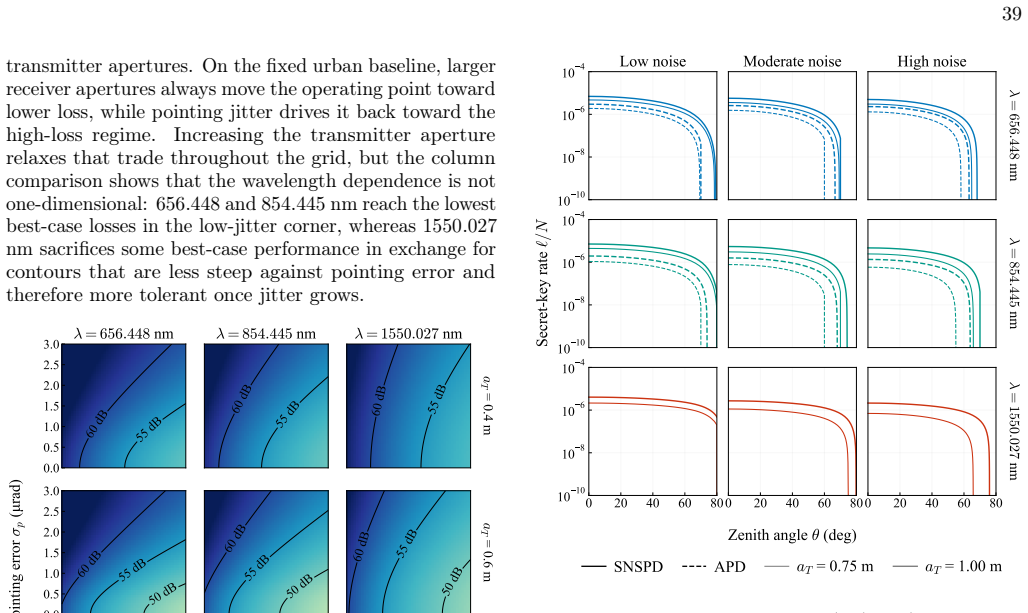
These effects increase the apparent beam radius at the receiver beyond its diffraction-limited value [80]
Turbulence This refers to irregular variations in the atmospheric refractive index, driven by temperature gradients, wind shear, pressure and humidity fluctuations, which per- turb the propagation of optical waves. These effects increase the apparent beam radius at the receiver beyond its diffraction-limited value [80]. In a satellite-to-ground downlink s...
-
[2]
Even with perfect alignment, a significant fraction of the transmitted beam power may fall outside the finite receiver aperture
Geometric loss Geometric loss, often referred to as aperture truncation loss, occurs because the optical beam spreads due to diffraction and atmospheric turbulence as it propagates. Even with perfect alignment, a significant fraction of the transmitted beam power may fall outside the finite receiver aperture. Assuming a circularly symmetric Gaussian inten...
-
[3]
This misalignment reduces the effective power coupled into the system
Pointing loss Pointing loss arises from the residual mechanical jitter of the transmitter, which causes random displacements of the beam centroid relative to the center of the receiver aperture [82]. This misalignment reduces the effective power coupled into the system. Modeling the pointing error as a Gaussian random vari- able with radial standard devia...
-
[4]
1 + aR r0 5/3#−6/5 ,(H34) wherer 0 is the Fried coherence parameter, given by r0 =
Coupling loss The coupling loss quantifies the fraction of transmitted optical power that falls outside the receiver field of view (FOV) and is not coupled into the detection system. In a free-space optical (FSO) receiver, the FOV defines the angular region over which the detector collects the in- coming light. The choice of FOV directly determines the tr...
-
[5]
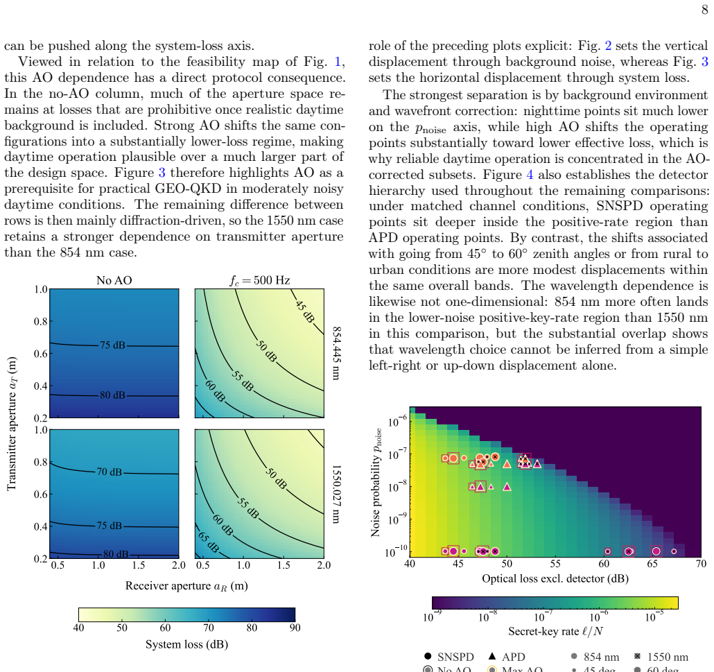
In this framework, AO correction is modeled as an effective enhancement of the Fried coherence value from its uncorrected valuer0 to a closed-loop corrected value rCL 0 > r0
Adaptive optics compensation Adaptive optics (AO) systems are implemented to re- duce turbulence-induced phase distortions by actively correcting phase aberrations across the receiver aperture [86]. In this framework, AO correction is modeled as an effective enhancement of the Fried coherence value from its uncorrected valuer0 to a closed-loop corrected v...
-
[6]
We note that the MODTRAN radiative transfer code [98] provides an alternative, widely used implementation with comparable capabilities
Absorption/scattering loss To model the channel loss arising from atmospheric ab- sorption and scattering processes, we employ a radiative transfer code, via thelibRadtran package [55, 56]. We note that the MODTRAN radiative transfer code [98] provides an alternative, widely used implementation with comparable capabilities. Both codes offer suites of stan...
2035
-
[7]
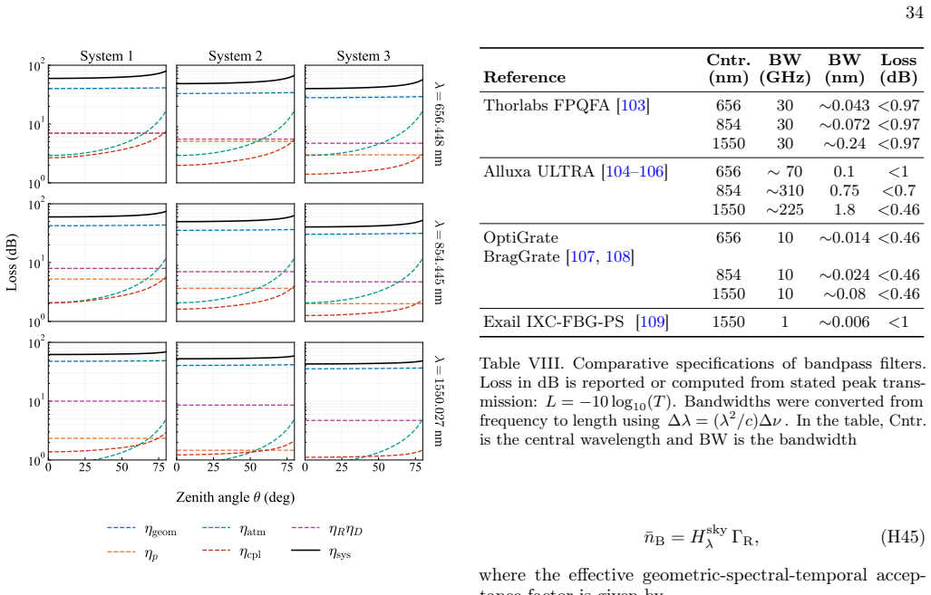
Overall system loss Combining all the effects detailed so far, the overall transmittance ηsys of the satellite downlink system is given by ηsys =η geoηpηcplηatmηRηD,(H44) where ηR denotes the total internal transmittance of the receiver subsystem excluding the single-photon detectors. This term captures the aggregate efficiency of the tele- scope optics (...
-
[8]
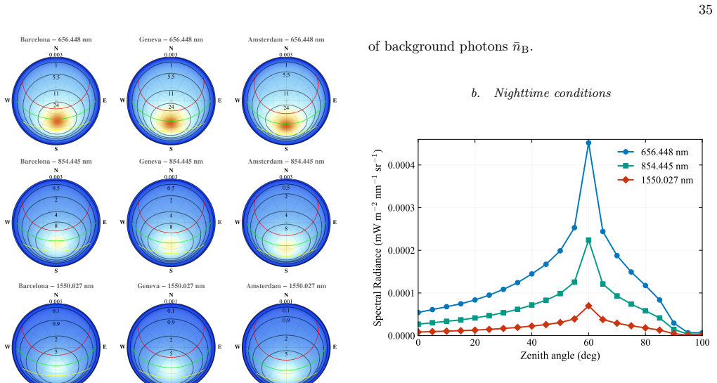
Background noise This subsection gives the explicit calculation of the mean background-photon level¯nB and the derived noise- click probability pnoise that define the nighttime and day- time noise scenarios used in Sec. V. For a receiver with angular field of viewΩFOV, using a detector within a temporal window∆t and a spectral filter of bandwidth∆λ center...
-
[9]
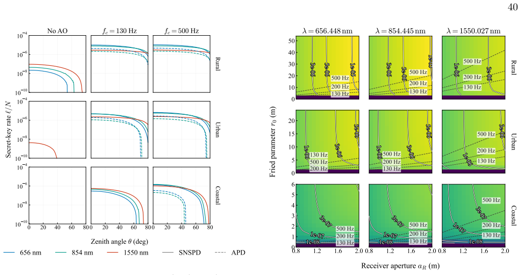
These scenarios are characterized by their altitude, visibility conditions, and atmospheric turbulence profiles, as summarized in Table II
Locations To assess the feasibility of GEO-QKD under diverse operational conditions, we consider three representative locations for the OGS that span a practical range of atmo- spheric environments. These scenarios are characterized by their altitude, visibility conditions, and atmospheric turbulence profiles, as summarized in Table II. The three location...
-
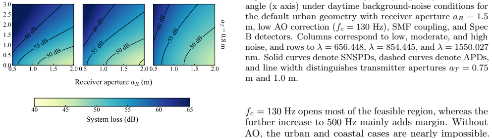
[10]
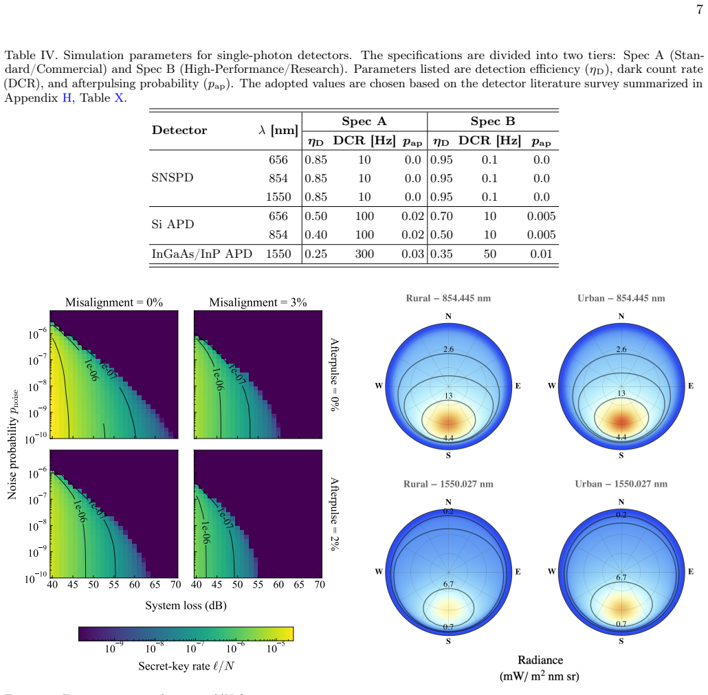
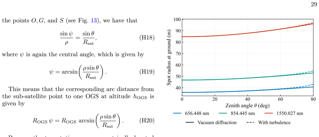
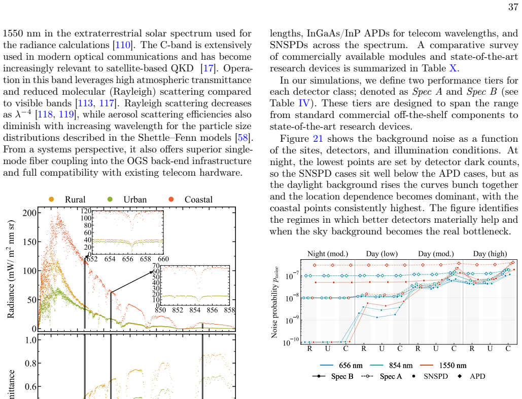
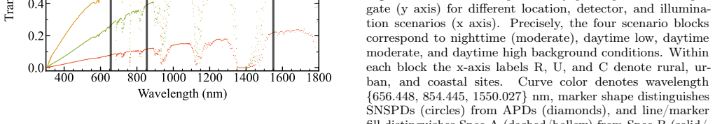
Wavelengths Wefocusonthreerepresentativewavelengths: 656.448nm (Hα line), 854.445 nm (Ca II line), and 1550.027 nm (C- band representative). The first two lie on prominent Fraunhofer lines in the solar spectrum, where the Sun it- self is significantly dimmer because a substantial fraction of the radiation at those wavelengths is absorbed before it leaves ...
-
[11]
We consider Si APDs for visible and near-infrared wave- lengths, InGaAs/InP APDs for telecom wavelengths, and SNSPDs across the spectrum
Single-photon detection The performance of a satellite-to-ground QKD link critically depends on the receiver’s detection hardware. We consider Si APDs for visible and near-infrared wave- lengths, InGaAs/InP APDs for telecom wavelengths, and SNSPDs across the spectrum. A comparative survey of commercially available modules and state-of-the-art research dev...
-
[12]
Misalignment Extensiveexperimentalandtheoreticalworkhasdemon- strated effective approaches for mitigating polarization misalignment in satellite-based QKD systems. In theMi- ciusmissions, active polarization control was implemented using reference laser pulses to monitor the evolving polar- ization state of the downlink channel, enabling real-time compens...
-
[13]
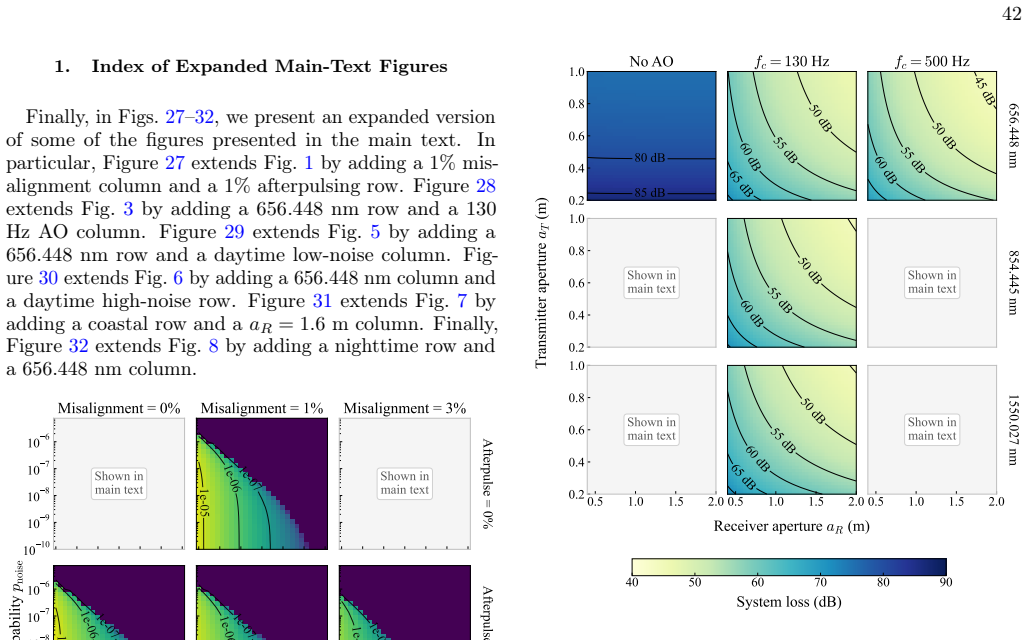
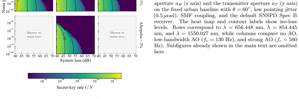
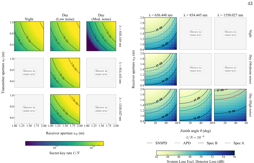
27–32, we present an expanded version of some of the figures presented in the main text
Index of Expanded Main-Text Figures Finally, in Figs. 27–32, we present an expanded version of some of the figures presented in the main text. In particular, Figure 27 extends Fig. 1 by adding a1%mis- alignment column and a1%afterpulsing row. Figure 28 extends Fig. 3 by adding a656.448nm row and a130 Hz AO column. Figure 29 extends Fig. 5 by adding a 656....
-
[14]
C. H. Bennett and G. Brassard, Quantum cryptography: Public key distribution and coin tossing, Theor. Comput. Sci.560, 7 (2014), originally published in Proceedings of IEEE International Conference on Computers, Systems and Signal Processing, Bangalore, India, 1984
2014
-
[15]
A. K. Ekert, Quantum cryptography based on Bell’s theorem, Phys. Rev. Lett.67, 661 (1991)
1991
-
[16]
H.-K. Lo, M. Curty, and K. Tamaki, Secure quantum key distribution, Nat. Photonics8, 595 (2014)
2014
-
[17]
Pirandola, U
S. Pirandola, U. L. Andersen, L. Banchi, M. Berta, D. Bunandar, R. Colbeck, D. Englund, T. Gehring, C. Lupo, C. Ottaviani,et al., Advances in quantum cryptography, Adv. Opt. Photonics12, 1012 (2020)
2020
-
[18]
F. Xu, X. Ma, Q. Zhang, H.-K. Lo, and J.-W. Pan, Secure quantum key distribution with realistic devices, Rev. Mod. Phys.92, 025002 (2020)
2020
-
[19]
H.-K. Lo, H. F. Chau, and M. Ardehali, Efficient quan- tum key distribution scheme and a proof of its uncondi- tional security, J. Cryptol.18, 133 (2005)
2005
-
[20]
Liuet al., 1002 km twin-field quantum key distribu- tion with finite-key analysis, Quantum Frontiers2, 16 (2023)
Y. Liuet al., 1002 km twin-field quantum key distribu- tion with finite-key analysis, Quantum Frontiers2, 16 (2023)
2023
-
[21]
J. S. Sidhu, S. K. Joshi,et al., Advances in space quan- tum communications, IET Quantum Commun.2, 182 (2021)
2021
-
[22]
Bedington, J
R. Bedington, J. M. Arrazola, and A. Ling, Progress in satellite quantum key distribution, npj Quantum Inf.3, 30 (2017)
2017
-
[23]
Liao, W.-Q
S.-K. Liao, W.-Q. Cai, W.-Y. Liu, L. Zhang, Y. Li, J.-G. Ren, J. Yin, Q. Shen, Y. Cao, Z.-P. Li,et al., Satellite- to-ground quantum key distribution, Nature549, 43 (2017)
2017
-
[24]
Liao, W.-Q
S.-K. Liao, W.-Q. Cai, J. Handsteiner, B. Liu, J. Yin, L. Zhang, D. Rauch, M. Fink, J.-G. Ren, W.-Y. Liu, et al.,Satellite-relayedintercontinentalquantumnetwork, Phys. Rev. Lett.120, 030501 (2018)
2018
-
[25]
Hwang, Quantum key distribution with high loss: Toward global secure communication, Phys
W.-Y. Hwang, Quantum key distribution with high loss: Toward global secure communication, Phys. Rev. Lett. 91, 057901 (2003)
2003
-
[26]
H.-K. Lo, X. Ma, and K. Chen, Decoy state quantum key distribution, Phys. Rev. Lett.94, 230504 (2005)
2005
-
[27]
Wang, Beating the photon-number-splitting attack in practical quantum cryptography, Phys
X.-B. Wang, Beating the photon-number-splitting attack in practical quantum cryptography, Phys. Rev. Lett.94, 230503 (2005)
2005
-
[28]
Li, S.-K
Y. Li, S.-K. Liao, Y. Cao, J.-G. Ren, W.-Y. Liu, J. Yin, Q. Shen, J.-C. Qiang, S. Zhang, A.-L. Jia,et al., Microsatellite-based real-time quantum key distribution, Nature640, 47 (2025)
2025
-
[29]
Liao, H.-L
S.-K. Liao, H.-L. Yong, C. Liu, G.-L. Shentu, D.-D. Li, J. Lin, H. Dai, S.-Q. Zhao, B. Li, J.-Y. Guan,et al., Long- distance free-space quantum key distribution in daylight towards inter-satellite communication, Nat. Photonics 11, 509 (2017)
2017
-
[30]
Avesani, L
M. Avesani, L. Calderaro, M. Schiavon, A. Stanco, C. Ag- nesi, A. Santamato, M. Zahidy, A. Scriminich, G. Fo- letto, G. Contestabile,et al., Full daylight quantum-key- distribution at 1550 nm enabled by integrated silicon photonics, npj Quantum Inf.7, 93 (2021)
2021
-
[31]
W.-Q. Cai, Y. Li, B. Li, J.-G. Ren, S.-K. Liao, Y. Cao, L. Zhang, M. Yang, J.-C. Wu, Y.-H. Li,et al., Free-space quantum key distribution during daylight and at night, Optica11, 647 (2024)
2024
-
[32]
Bourgoin, E
J.-P. Bourgoin, E. Meyer-Scott, B. L. Higgins, B. Helou, C. Erven, H. Hübel, B. Kumar, D. Hudson, I. D’Souza, R. Girard,et al., A comprehensive design and perfor- mance analysis of low Earth orbit satellite quantum communication, New J. Phys.15, 023006 (2013)
2013
-
[33]
J. S. Sidhu, T. Brougham, D. McArthur, R. G. Pousa, and D. K. Oi, Finite key performance of satellite quan- tum key distribution under practical constraints, Com- mun. Phys.6, 210 (2023)
2023
-
[34]
Vasylyev, W
D. Vasylyev, W. Vogel, and F. Moll, Satellite-mediated quantum atmospheric links, Phys. Rev. A99, 053830 (2019)
2019
-
[35]
Liege, P
T. Liege, P. Lognoné, M. Schiavon, C. B. Lim, J.-M. Co- nan, E. Diamanti, and D. Dequal, Analysis of untrusted- node quantum key distribution from a geostationary satellite, Quantum Sci. Technol.11, 025002 (2026)
2026
-
[36]
Xin, China’s new Dawn: Pan Jianwei reveals high- orbit quantum satellite for global network, South China Morning Post (2025), [Online; accessed 2026-01-16]
L. Xin, China’s new Dawn: Pan Jianwei reveals high- orbit quantum satellite for global network, South China Morning Post (2025), [Online; accessed 2026-01-16]. Announcement at 2024 Zhongguancun Forum, Beijing
2025
-
[37]
Dirks, I
B. Dirks, I. Ferrario, A. Le Pera, D. V. Finocchiaro, M. Desmons, D. de Lange, H. de Man, A. J. Meskers, J. Morits, N. M. Neumann,et al., GEOQKD: quantum key distribution from a geostationary satellite, inInter- national Conference on Space Optics—ICSO 2020, Vol. 11852 (SPIE, 2021) p. 222
2020
-
[38]
W. Klop, R. Saathof, N. Doelman, M. Gruber, T. Moens, C. I. O. Tamayo, and C. Duque, QKD optical ground terminal developments, inInternational Conference on Space Optics—ICSO 2020, Vol. 11852 (SPIE, 2021) p. 388
2020
-
[39]
Hispasat, Hispasat and ESA agree to develop the first QKD system combining the delivery of quantum keys from GEO and LEO orbits (2025), [Online; accessed 2026-05-15]
2025
-
[40]
A. Abad, P. Pintó, F. Cuervo, Á. Álvaro, L. Pascual, J. C. Gil, V. Gaspar, J. Autrán, L. F. Rodríguez, M. Reyes García-Talavera, L. Trigo Vidarte, V. Pruneri, D. Domingo, M. I. García, A. Álvarez-Herrero, T. Be- lenger, V. Fernandez, P. Arteaga-Díaz, D. Cano, J. Sanz, C. Miravet, P. Campo, J. Bermejo, M. Curty, V. Martín, J. P. Brito, and L. Ortíz, Quantu...
2022
-
[41]
Alvaro, L
A. Alvaro, L. Pascual, T. Colombo, M. Guerault, and V. Giner, GARBO QKD GEO: challenges and ar- chitecture, inInternational Conference on Space Op- tics—ICSO 2024, Vol. 13699 (SPIE, 2025) p. 1527
2024
-
[42]
Pirandola, Satellite quantum communications: Fun- damental bounds and practical security, Phys
S. Pirandola, Satellite quantum communications: Fun- damental bounds and practical security, Phys. Rev. Res. 3, 023130 (2021)
2021
-
[43]
Pirandola, Limits and security of free-space quantum communications, Phys
S. Pirandola, Limits and security of free-space quantum communications, Phys. Rev. Res.3, 013279 (2021)
2021
-
[44]
Günthner, I
K. Günthner, I. Khan,et al., Quantum-limited measure- ments of optical signals from a geostationary satellite, Optica4, 611 (2017)
2017
-
[45]
C. C. W. Lim, M. Curty, N. Walenta, F. Xu, and H. Zbinden, Concise security bounds for practical decoy- state quantum key distribution, Phys. Rev. A89, 022307 46 (2014)
2014
-
[46]
R. J. Serfling, Probability inequalities for the sum in sampling without replacement, Ann. Stat.2, 39 (1974)
1974
-
[47]
Hoeffding, Probability inequalities for sums of bounded random variables, J
W. Hoeffding, Probability inequalities for sums of bounded random variables, J. Am. Stat. Assoc.58, 13 (1963)
1963
-
[48]
Curty, F
M. Curty, F. Xu, W. Cui, C. C. W. Lim, K. Tamaki, and H.-K. Lo, Finite-key analysis for measurement-device- independent quantum key distribution, Nat. Commun. 5, 3732 (2014)
2014
-
[49]
Zhang, Q
Z. Zhang, Q. Zhao, M. Razavi, and X. Ma, Improved key-rate bounds for practical decoy-state quantum-key- distribution systems, Phys. Rev. A95, 012333 (2017)
2017
-
[50]
Attema, J
T. Attema, J. W. Bosman, and N. M. Neumann, Opti- mizing the decoy-state BB84 QKD protocol parameters, Quantum Inf. Process.20, 154 (2021)
2021
-
[51]
J.-D. Bancal and P. Sekatski, Simple Buehler-optimal confidence intervals on the average success probabil- ity of independent Bernoulli trials, arXiv preprint arXiv:2212.12558 (2022)
-
[52]
Mannalath, V
V. Mannalath, V. Zapatero, and M. Curty, Sharp finite statistics for quantum key distribution, Phys. Rev. Lett. 135, 020803 (2025)
2025
-
[53]
Elementary Tail Bounds on the Hypergeometric Distribution
V. Mannalath, V. Zapatero, and M. Curty, Elementary Tail Bounds on the Hypergeometric Distribution, arXiv preprint arXiv:2510.19726 (2025)
work page internal anchor Pith review Pith/arXiv arXiv 2025
-
[54]
Tomamichel, C
M. Tomamichel, C. C. W. Lim, N. Gisin, and R. Renner, Tight finite-key analysis for quantum cryptography, Nat. Commun.3, 634 (2012)
2012
-
[55]
Phys.14, 093014 (2012)
M.HayashiandT.Tsurumaru,Conciseandtightsecurity analysis of the Bennett–Brassard 1984 protocol with finite key lengths, New J. Phys.14, 093014 (2012)
1984
-
[56]
Tupkary, S
D. Tupkary, S. Nahar, P. Sinha, and N. Lütkenhaus, Phase error rate estimation in QKD with imperfect de- tectors, Quantum9, 1937 (2025)
1937
-
[57]
Tupkary, E
D. Tupkary, E. Y.-Z. Tan, and N. Lütkenhaus, Security proof for variable-length quantum key distribution, Phys. Rev. Res.6, 023002 (2024)
2024
- [58]
-
[59]
Tzallas, A
V. Tzallas, A. Hünerbein, M. Stengel, J. F. Meirink, N. Benas, J. Trentmann, and A. Macke, CRAAS: a European cloud regime dAtAset based on the CLAAS- 2.1 climate data record, Remote Sens.14, 5548 (2022)
2022
-
[60]
Wright,Exact confidence bounds when sampling from small finite universes: an easy reference based on the hypergeometric distribution, Lecture Notes in Statistics, Vol
T. Wright,Exact confidence bounds when sampling from small finite universes: an easy reference based on the hypergeometric distribution, Lecture Notes in Statistics, Vol. 66 (Springer New York, 1991)
1991
-
[61]
A. E. Siegman,Lasers(University Science Books, 1986)
1986
-
[62]
A. E. Siegman, Defining, measuring, and optimizing laser beam quality, SPIE Proceedings1868, 2 (1993)
1993
-
[63]
R.HufnagelandN.Stanley,Modulationtransferfunction associated with image transmission through turbulent media, J. Opt. Soc. Am.54, 52 (1964)
1964
-
[64]
G. C. Valley, Isoplanatic degradation of tilt correction and short-term imaging systems, Appl. Opt.19, 574 (1980)
1980
-
[65]
J. W. Hardy,Adaptive optics for astronomical telescopes, Vol. 16 (Oxford University Press, USA, 1998)
1998
-
[66]
C. J. Pugh, J.-F. Lavigne, J.-P. Bourgoin, B. L. Higgins, and T. Jennewein, Adaptive optics benefit for quantum key distribution uplink from ground to a satellite, Adv. Opt. Technol.9, 263 (2020)
2020
-
[67]
R. N. Lanning, M. A. Harris, D. W. Oesch, M. D. Oliker, and M. T. Gruneisen, Quantum communication over atmospheric channels: a framework for optimizing wave- length and filtering, Phys. Rev. Appl.16, 044027 (2021)
2021
-
[68]
C. Emde, R. Buras-Schnell, A. Kylling, B. Mayer, J. Gasteiger, U. Hamann, J. Kylling, B. Richter, C. Pause, T. Dowling,et al., The libRadtran software package for radiative transfer calculations (version 2.0.1), Geosci. Model Dev.9, 1647 (2016)
2016
-
[69]
Mayer and A
B. Mayer and A. Kylling, Technical note: The libRad- tran software package for radiative transfer calculations - description and examples of use, Atmos. Chem. Phys. 5, 1855 (2005)
2005
-
[70]
United States Committee on Extension to the Standard Atmosphere,US standard atmosphere, 1976(National Oceanic and Atmospheric Administration, 1976)
1976
-
[71]
E. P. Shettle and R. W. Fenn,Models for the aerosols of the lower atmosphere and the effects of humidity varia- tions on their optical properties, AFGL Technical Report AFGL-TR-79-0214 (Air Force Geophysics Laboratory, Air Force Systems Command, United States Air Force, Hanscom AFB, MA, 1979) Environmental Research Pa- pers No. 676, 94 pp
1979
-
[72]
E. P. Shettle, Models of aerosols, clouds, and precipita- tion for atmospheric propagation studies, inAtmospheric Propagation in the UV, Visible, IR and MM-Wave Re- gion and Related Systems Aspects, AGARD Conference Proceedings No. 454 (Advisory Group for Aerospace Re- search and Development, Copenhagen, Denmark, 1990) pp. 15–1–15–13
1990
-
[73]
Finkensieper, J
S. Finkensieper, J. F. Meirink, G.-J. van Zadelhoff, T. Hanschmann, N. Benas, M. Stengel, P. Fuchs, R. Holl- mann, J. Kaiser, and M. Werscheck, CLAAS-2.1: CM SAFCLoudpropertydAtAsetusingSEVIRI-Edition2.1 (2020), dataset, Satellite Application Facility on Climate Monitoring (CM SAF); [Online; accessed 2025-10-22]
2020
-
[74]
ESO, Sky Model Calculator (n.d.), [Online; accessed 2026-05-15]
2026
-
[75]
S. Noll, W. Kausch, M. Barden, A. Jones, C. Szyszka, S. Kimeswenger, and J. Vinther, An atmospheric radi- ation model for Cerro Paranal-I. The optical spectral range, Astron. Astrophys.543, A92 (2012)
2012
-
[76]
Jones, S
A. Jones, S. Noll, W. Kausch, C. Szyszka, and S.Kimeswenger,Anadvancedscatteredmoonlightmodel for Cerro Paranal, Astron. Astrophys.560, A91 (2013)
2013
-
[77]
J. S. Sidhu, T. Brougham, D. McArthur, R. G. Pousa, and D. K. L. Oi, Finite key effects in satellite quantum key distribution, npj Quantum Inf.8, 18 (2022)
2022
-
[78]
Pirandola, R
S. Pirandola, R. Laurenza, C. Ottaviani, and L. Banchi, Fundamental limits of repeaterless quantum communi- cations, Nat. Commun.8, 15043 (2017)
2017
-
[79]
Pirandola, End-to-end capacities of a quantum com- munication network, Commun
S. Pirandola, End-to-end capacities of a quantum com- munication network, Commun. Phys.2, 51 (2019)
2019
-
[80]
Azuma, S
K. Azuma, S. E. Economou, D. Elkouss, P. Hilaire, L. Jiang, H.-K. Lo, and I. Tzitrin, Quantum repeaters: From quantum networks to the quantum internet, Rev. Mod. Phys.95, 045006 (2023)
2023
discussion (0)
Sign in with ORCID, Apple, or X to comment. Anyone can read and Pith papers without signing in.