Koopman--von Neumann Molecular Dynamics for Green--Kubo Transport Coefficients
Pith reviewed 2026-06-29 07:18 UTC · model grok-4.3
The pith
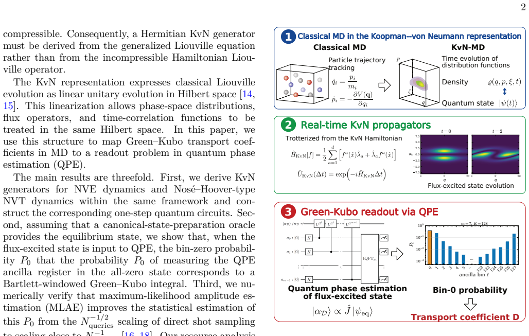
The Koopman-von Neumann representation turns classical molecular dynamics into unitary quantum evolutions so Green-Kubo transport coefficients become quantum phase estimation readouts.
A machine-rendered reading of the paper's core claim, the machinery that carries it, and where it could break.
Core claim
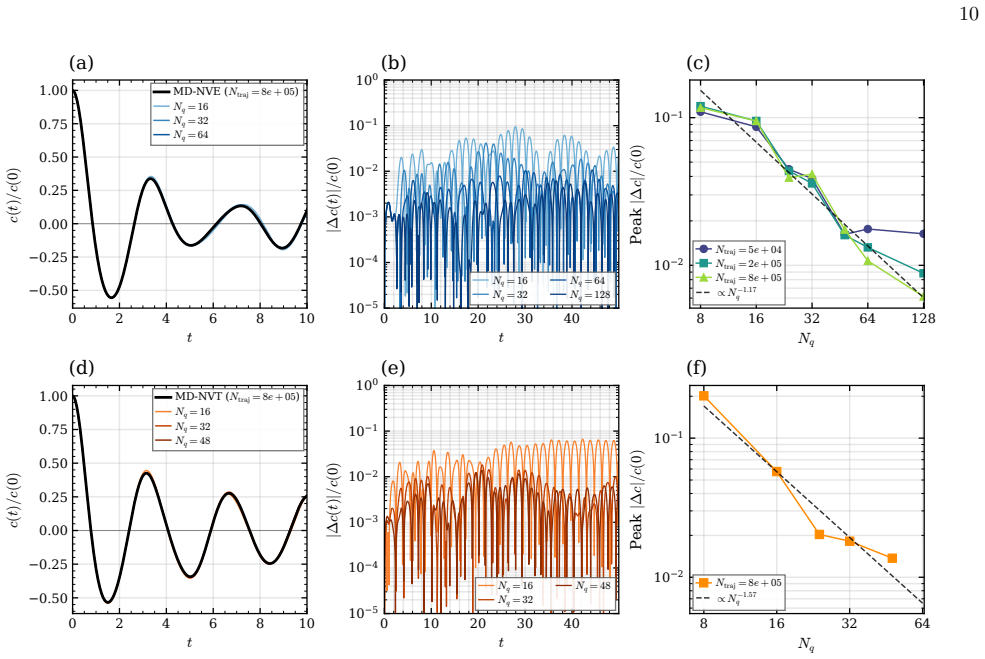
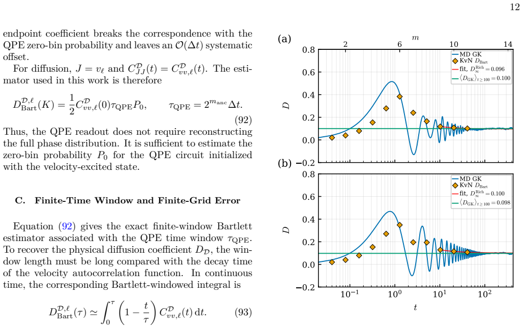
Both NVE and Nosé-Hoover-type NVT dynamics are derived as unitary evolutions on Hilbert spaces associated with the corresponding classical phase spaces. Numerical benchmarks on finite grids show that the discretization error in the correlation function decreases as a power law in the number of grid points Nz. Equivalently, with Nz=2^nz the error decreases exponentially in the register size nz. To read out a transport coefficient, a flux-excited state is input to quantum phase estimation; the probability P0 of measuring the ancilla register in the all-zero state corresponds to a Bartlett-windowed Green-Kubo integral. With maximum-likelihood amplitude estimation the statistical estimation of P
What carries the argument
The Koopman-von Neumann representation, which associates classical phase-space functions with vectors in a Hilbert space so that the classical time-evolution operator becomes a unitary operator on that space.
If this is right
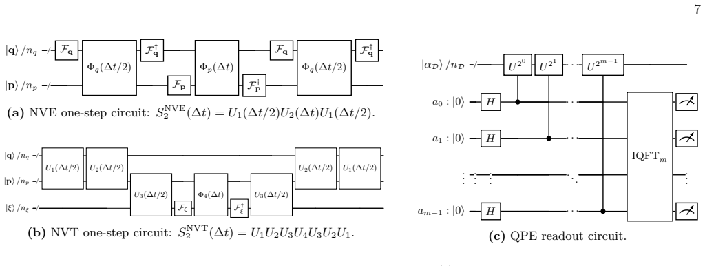
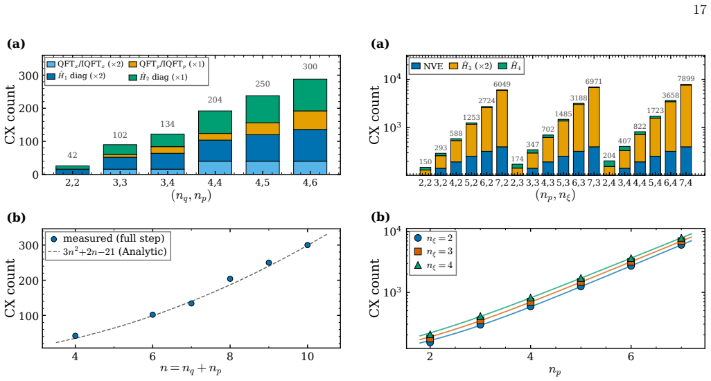
- One step of the NVE propagator can be implemented with O(n^2) CX gates where n equals the total number of position and momentum qubits.
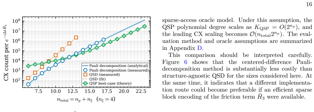
- The centered-difference implementation of the Nosé-Hoover friction term for NVT scales as O(n_ξ n_p 2^{n_p}).
- A target accuracy ε for the transport coefficient requires only O(log(1/ε)) qubits for the grid register.
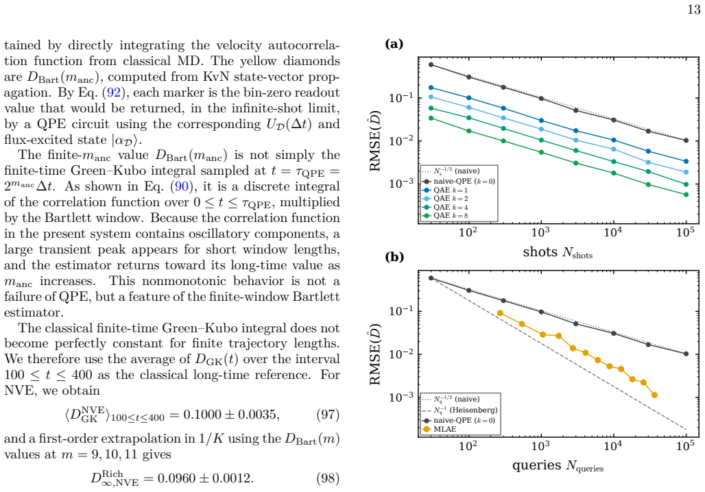
- Maximum-likelihood amplitude estimation applied to the QPE oracle yields statistical scaling close to N_queries^{-1} rather than the direct-sampling N_queries^{-1/2}.
Where Pith is reading between the lines
- The same unitary-lifting construction could be applied to other classical statistical-mechanical ensembles whose propagators admit a phase-space representation.
- Hybrid algorithms that interleave the KvN propagator with existing quantum Hamiltonian-simulation routines might allow larger phase-space grids without increasing qubit count proportionally.
- The logarithmic qubit scaling assumes the power-law convergence continues to arbitrarily fine grids; practical limits set by floating-point precision or memory would cap the achievable accuracy on current hardware.
Load-bearing premise
The finite-grid discretization of the classical phase space produces a unitary operator whose long-time correlation functions converge to the continuous Green-Kubo integrals at a power-law rate in the number of grid points.
What would settle it
A numerical test on successively refined grids in which the measured correlation-function error fails to decrease as a power law with Nz or deviates systematically from the classical integral outside statistical fluctuations.
Figures
read the original abstract
We formulate the Green--Kubo transport coefficients of classical molecular dynamics as a readout problem for quantum algorithms using the Koopman--von Neumann (KvN) representation. Both NVE and Nos\'e--Hoover-type NVT dynamics are derived as unitary evolutions on Hilbert spaces associated with the corresponding classical phase spaces. Numerical benchmarks on finite grids show that the discretization error in the correlation function decreases as a power law in the number of grid points $N_z$. Equivalently, with $N_z=2^{n_z}$, the error decreases exponentially in the register size $n_z$, so a target accuracy $\epsilon$ requires $n_z=\mathcal{O}(\log(1/\epsilon))$ qubits. To read out a transport coefficient, we input a flux-excited state to quantum phase estimation (QPE). The probability $P_0$ of measuring the QPE ancilla register in the all-zero state corresponds to a Bartlett-windowed Green--Kubo integral. With maximum-likelihood amplitude estimation, the statistical estimation of $P_0$ defined by this QPE oracle improves from the $N_{\rm queries}^{-1/2}$ scaling of direct shot sampling to scaling close to $N_{\rm queries}^{-1}$. Our circuit-resource analysis shows that one step of the NVE propagator can be built with $\mathcal{O}(n^2)$ CX gates, where $n=n_x+n_p$ is the total number of position and momentum qubits. For the NVT propagator, the centered-difference Pauli-decomposition implementation of the Nos\'e--Hoover friction term scales as $\mathcal{O}(n_\xi n_p\,2^{n_p})$, where $n_p$ and $n_\xi$ are the numbers of momentum and thermostat qubits, respectively. The proposed framework is a concrete step toward translating the principles of quantum algorithms into the transport-coefficient calculations required in practical molecular simulation.
Editorial analysis
A structured set of objections, weighed in public.
Referee Report
Summary. The paper formulates Green-Kubo transport coefficients of classical molecular dynamics as a quantum readout problem via the Koopman-von Neumann (KvN) representation. It derives unitary evolutions on associated Hilbert spaces for both NVE and Nosé-Hoover NVT dynamics, reports numerical benchmarks showing power-law decay of discretization error in correlation functions with grid size N_z (hence exponential decay in qubit number n_z = log2(N_z)), and proposes using quantum phase estimation (QPE) on a flux-excited state with maximum-likelihood amplitude estimation to extract a Bartlett-windowed integral of the correlation function. Circuit-resource estimates are given for the propagators.
Significance. If the discretization convergence holds, the work supplies a concrete mapping from classical transport-coefficient calculations to quantum algorithms, with explicit O(n^2) CX scaling for the NVE step and an amplitude-estimation improvement from N_queries^{-1/2} to near N_queries^{-1}. The numerical benchmarks on small grids and the parameter-free character of the KvN-to-quantum mapping are positive features.
major comments (1)
- [Abstract] Abstract (discretization benchmarks paragraph): the headline claim that n_z = O(log(1/ε)) suffices for target accuracy ε rests on the finite-grid unitary U_{N_z} producing correlation functions whose time integrals converge to the continuous Green-Kubo value at a power-law rate in N_z. Only numerical benchmarks on small grids are reported; no operator-norm bound, weak-convergence argument, or analysis establishing that the grid KvN propagator approximates the continuous Liouville evolution in the topology required for ∫C(t)dt as N_z→∞ and t→∞ simultaneously is supplied. This assumption is load-bearing for both the qubit scaling and the subsequent QPE readout argument.
Simulated Author's Rebuttal
We thank the referee for their careful reading and for identifying this key assumption in our work. We respond to the major comment below.
read point-by-point responses
-
Referee: [Abstract] Abstract (discretization benchmarks paragraph): the headline claim that n_z = O(log(1/ε)) suffices for target accuracy ε rests on the finite-grid unitary U_{N_z} producing correlation functions whose time integrals converge to the continuous Green-Kubo value at a power-law rate in N_z. Only numerical benchmarks on small grids are reported; no operator-norm bound, weak-convergence argument, or analysis establishing that the grid KvN propagator approximates the continuous Liouville evolution in the topology required for ∫C(t)dt as N_z→∞ and t→∞ simultaneously is supplied. This assumption is load-bearing for both the qubit scaling and the subsequent QPE readout argument.
Authors: We agree that the headline qubit scaling n_z = O(log(1/ε)) is supported only by the reported numerical benchmarks on small grids showing power-law decay of discretization error in the correlation functions, rather than by a rigorous operator-norm bound or weak-convergence analysis of the discretized KvN propagator in the topology needed for the integrated Green-Kubo quantity under the joint limits N_z o ∞ and t o ∞. The manuscript presents these benchmarks as empirical evidence but does not claim or supply such a proof. We will revise the abstract to state explicitly that the power-law convergence (and consequent logarithmic qubit scaling) is observed in numerical benchmarks on finite grids, and we will add a brief discussion noting that a rigorous continuum-limit analysis remains an open question for future work. This revision will be made to ensure the load-bearing assumption is presented accurately. revision: yes
Circularity Check
No significant circularity; derivation is a direct mapping with numerical support
full rationale
The paper constructs a formulation mapping classical Green-Kubo integrals to quantum readout via KvN unitary operators on discretized phase space, derives the NVE/NVT propagators explicitly, and reports numerical power-law decay of discretization error in correlation functions to support the logarithmic qubit claim. No equation reduces the target transport coefficient to a fitted input by construction, no self-citation is load-bearing for the central claim, and the discretization convergence is presented as an observed benchmark rather than an unverified self-referential assumption. The chain remains independent of its own outputs.
Axiom & Free-Parameter Ledger
axioms (1)
- domain assumption The Koopman-von Neumann representation maps classical phase-space functions to operators on a Hilbert space such that the Liouville operator becomes a Hermitian operator generating unitary evolution.
Reference graph
Works this paper leans on
-
[1]
(A1) The coordinate q is a physically periodic variable
T est Model and Error Metric For the test system, we use the one-dimensional cosine potential V (q) = V0 cos q, q 2 [0, 2π). (A1) The coordinate q is a physically periodic variable. By contrast, the momentum p and the Nosé–Hoover variable ξ are nonperiodic variables and are numerically truncated to the finite intervals p 2 [pmax, pmax), ξ 2 [ξmax, ξmax). ...
-
[2]
By contrast, the p and ξ axes are intrinsically nonperiodic
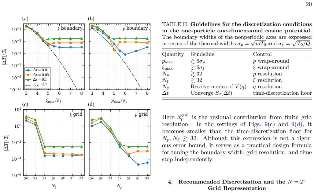
Boundaries of Nonperiodic Axes and W rap-Around Error The q axis is physically periodic and is therefore com- patible with Fourier differentiation. By contrast, the p and ξ axes are intrinsically nonperiodic. When Fourier differentiation is used on a finite grid, however, these fi- nite intervals are numerically treated as periodically con- nected. Conseq...
-
[3]
Figures 9(c) and 9(d) show the results obtained by fixing either ξmax or pmax to 8σ and varying Nξ and Np
Grid Resolution and the Time-Discretization Floor After the boundary width is made sufficiently large, the remaining errors are controlled by the number of grid points and the time step. Figures 9(c) and 9(d) show the results obtained by fixing either ξmax or pmax to 8σ and varying Nξ and Np. In the low-resolution regime, even when the Gaussian tail is con...
-
[4]
K + 2 K−1X s=1 (K s)cD(s∆t) # . (B13) Finally, multiplying Eq. ( B13) by 1 2 C (D) JJ (0)τQPE and using τQPE = K∆t, we obtain 1 2 C (D) JJ (0)τQPEP0 = C (D) JJ (0)∆t
Recommended Discretization and the N = 2 n Grid Representation Table II summarizes the practical discretization con- ditions inferred from Fig. 9 for the one-particle one- dimensional cosine potential. These values are represen- tative for the present model. Systems with stiffer poten- tials, lower-temperature distributions, or longer correla- tion times ...
-
[5]
For a diffusion coefficient, setting CJJ = Cvv gives Eq
The window vanishes at s = K, so no endpoint contri- bution appears there. For a diffusion coefficient, setting CJJ = Cvv gives Eq. ( 92) in the main text. 22 Appendix C: Details of the Centered-Difference Pauli-Decomposition Method This appendix summarizes the centered-difference Pauli-decomposition method used in Sec. VII A. The tar- get operator is the ...
1918
-
[6]
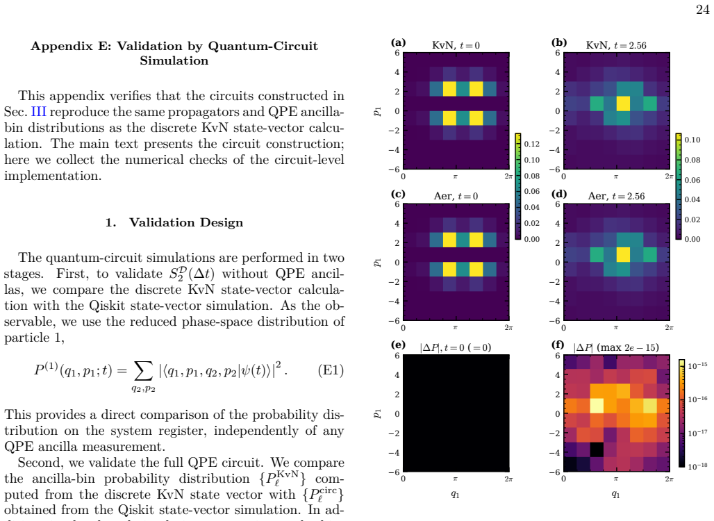
First, to validate SD 2 (∆t) without QPE ancil- las, we compare the discrete KvN state-vector calcula- tion with the Qiskit state-vector simulation
V alidation Design The quantum-circuit simulations are performed in two stages. First, to validate SD 2 (∆t) without QPE ancil- las, we compare the discrete KvN state-vector calcula- tion with the Qiskit state-vector simulation. As the ob- servable, we use the reduced phase-space distribution of particle 1, P (1)(q1, p1; t) = X q2,p2 jhq1, p1, q2, p2jψ(t)...
-
[7]
For the system register composed of the q and p registers of each particle, we repeatedly apply the same one-step propa- gator and evaluate P (1)(q1, p1; t) at t = 2 .56
Agreement of Reduced Phase-Space Distributions Figure 10 compares the reduced phase-space distribu- tions for the two-particle coupled cosine system. For the system register composed of the q and p registers of each particle, we repeatedly apply the same one-step propa- gator and evaluate P (1)(q1, p1; t) at t = 2 .56. The dis- tributions obtained from th...
-
[8]
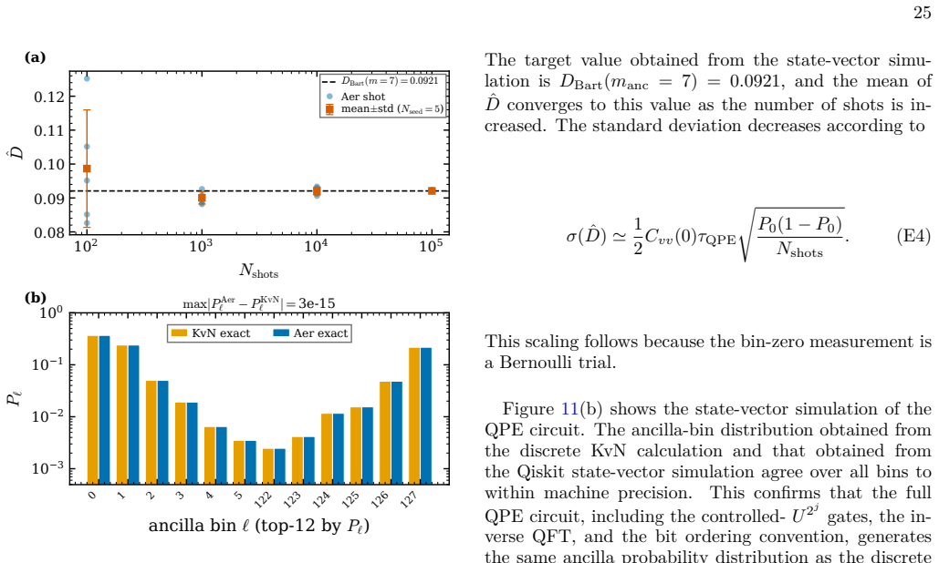
Here we use manc = 7 , corresponding to K = 2 7
QPE Ancilla-Bin Distribution and Finite-Shot Statistics Figure 11(a) shows the convergence of ˆD when the same QPE circuit is executed with a finite number of shots. Here we use manc = 7 , corresponding to K = 2 7. Since ∆t = 0.02, τQPE = K∆t = 2 manc ∆t = 2.56. (E3) 25 102 103 104 105 Nshots 0.08 0.09 0.10 0.11 0.12 ^D (a) DBart(m = 7) = 0:0921 Aer shot ...
-
[9]
M. E. Tuckerman, Statistical Mechanics: Theory and Molecular Simulation (Oxford University Press, 2023)
2023
-
[10]
Fallahzadeh and N
R. Fallahzadeh and N. Farhadian, Solid State Ionics 280, 10 (2015)
2015
-
[11]
Baktash, J
A. Baktash, J. C. Reid, T. Roman, and D. J. Searles, npj Computational Materials 6, 162 (2020)
2020
-
[12]
Muralidharan, M
A. Muralidharan, M. I. Chaudhari, L. R. Pratt, and S. B. Rempe, Scientific Reports 8, 10736 (2018)
2018
-
[13]
Kassal, S
I. Kassal, S. P. Jordan, P. J. Love, M. Mohseni, and A. Aspuru-Guzik, Proc. Natl. Acad. Sci. U.S.A. 105, 18681 (2008)
2008
-
[14]
J. D. Whitfield, J. Biamonte, and A. Aspuru-Guzik, Mol. Phys. 109, 735 (2011)
2011
-
[15]
Y. Su, D. W. Berry, N. Wiebe, N. Rubin, and R. Bab- bush, PRX Quantum 2, 040332 (2021)
2021
-
[16]
P. J. Ollitrault, A. Miessen, and I. Tavernelli, Acc. Chem. Res. 54, 4229 (2021)
2021
-
[17]
Joseph, Phys
I. Joseph, Phys. Rev. Research 2, 043102 (2020)
2020
-
[18]
Simon, R
S. Simon, R. Santagati, M. Degroote, N. Moll, M. Streif, and N. Wiebe, PRX Quantum 5, 010343 (2024)
2024
-
[19]
Fullqubit alchemist: Quantum algorithm for alchemical free energy calculations
P.-W. Huang, G. Boyd, G.-L. R. Anselmetti, M. De- groote, N. Moll, R. Santagati, M. Streif, B. Ries, D. Marti-Dafcik, H. Jnane, S. Simon, N. Wiebe, T. R. Bromley, and B. Koczor, arXiv arXiv:2508.16719, 10.48550/arXiv.2508.16719 (2025), arXiv:2508.16719
work page internal anchor Pith review Pith/arXiv arXiv doi:10.48550/arxiv.2508.16719 2025
-
[20]
S. Nosé, J. Chem. Phys. 81, 511 (1984)
1984
-
[21]
W. G. Hoover, Phys. Rev. A 31, 1695 (1985)
1985
-
[22]
B. O. Koopman, Proc. Natl. Acad. Sci. U.S.A. 17, 315 (1931)
1931
-
[23]
J. v. Neumann, Annals of Mathematics 33, 587 (1932)
1932
-
[24]
Brassard, P
G. Brassard, P. Høyer, M. Mosca, and A. Tapp, in Quantum Computation and Information , Contemporary Mathematics, Vol. 305 (American Mathematical Society,
-
[25]
Suzuki, S
Y. Suzuki, S. Uno, R. Raymond, T. Tanaka, T. Onodera, and N. Yamamoto, Quantum Inf. Process. 19, 75 (2020)
2020
-
[26]
Grinko, J
D. Grinko, J. Gacon, C. Zoufal, and S. Woerner, npj Quantum Inf. 7, 52 (2021)
2021
-
[27]
D. I. Bondar, F. Gay-Balmaz, and C. Tronci, Proc. R. Soc. A 475, 20180879 (2019)
2019
-
[28]
G. J. Martyna, M. L. Klein, and M. Tuckerman, J. Chem. Phys. 97, 2635 (1992)
1992
-
[29]
H. F. Trotter, Proceedings of the American Mathematical Society 10, 545 (1959) . 26
1959
-
[30]
Suzuki, Communications in Mathematical Physics 51, 183 (1976)
M. Suzuki, Communications in Mathematical Physics 51, 183 (1976)
1976
-
[31]
Suzuki, Phys
M. Suzuki, Phys. Lett. A 146, 319 (1990)
1990
-
[32]
Yoshida, Phys
H. Yoshida, Phys. Lett. A 150, 262 (1990)
1990
-
[33]
I. D. Kivlichan, C. Gidney, D. W. Berry, N. Wiebe, J. McClean, W. Sun, Z. Jiang, N. Rubin, A. Fowler, A. Aspuru-Guzik, H. Neven, and R. Babbush, Quantum 4, 296 (2020)
2020
-
[34]
Welch, D
J. Welch, D. Greenbaum, S. Mostame, and A. Aspuru- Guzik, New J. Phys. 16, 033040 (2014)
2014
-
[35]
Leimkuhler and C
B. Leimkuhler and C. Matthews, J. Chem. Phys. 138, 174102 (2013)
2013
-
[36]
A. Javadi-Abhari, M. Treinish, K. Krsulich, C. J. Wood, J. Lishman, J. Gacon, S. Martiel, P. D. Nation, L. S. Bishop, A. W. Cross, B. R. Johnson, and J. M. Gambetta, Quantum computing with Qiskit (2024), arXiv:2405.08810 [quant-ph]
work page internal anchor Pith review Pith/arXiv arXiv 2024
-
[37]
C. Z. Cheng and G. Knorr, J. Comput. Phys. 22, 330 (1976)
1976
-
[38]
A. J. Klimas, J. Comput. Phys. 68, 202 (1987)
1987
-
[39]
A. J. Klimas and W. M. Farrell, J. Comput. Phys. 110, 150 (1994)
1994
-
[40]
G. V. Vogman, P. Colella, and U. Shumlak, J. Comput. Phys. 277, 101 (2014)
2014
-
[41]
V. V. Shende, S. S. Bullock, and I. L. Markov, IEEE Trans. Comput.-Aided Des. Integr. Circuits Syst. 25, 1000 (2006)
2006
-
[42]
A. M. Childs and N. Wiebe, Quantum Inf. Comput. 12, 901 (2012)
2012
-
[43]
G. H. Low and I. L. Chuang, Quantum 3, 163 (2019)
2019
discussion (0)
Sign in with ORCID, Apple, or X to comment. Anyone can read and Pith papers without signing in.