Faithful Embeddings of Irregular and Asynchronous Data for Online Log-NCDEs
Pith reviewed 2026-06-29 08:56 UTC · model grok-4.3
The pith
Compact-set universality transfers from model input space to irregular data space if the embedding is continuous and injective.
A machine-rendered reading of the paper's core claim, the machinery that carries it, and where it could break.
Core claim
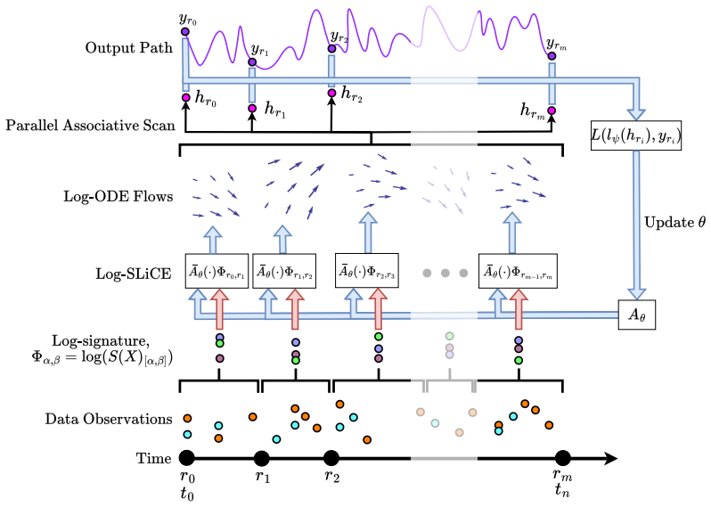
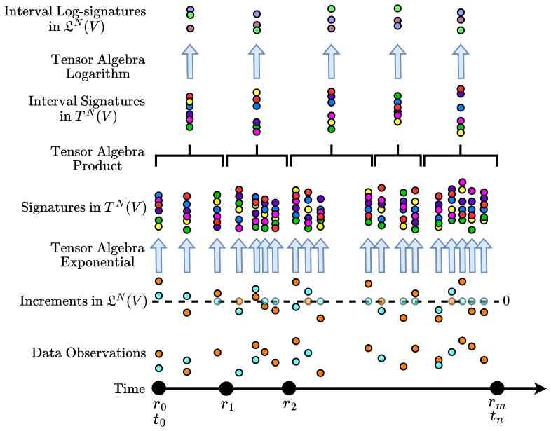
Under mild conditions, compact-set universality on the model input space transfers to the data space whenever the embedding from data to input is continuous and injective. Guided by this result, and building on the rectilinear control path for Neural Controlled Differential Equations (NCDEs), the authors introduce a continuous and injective embedding for Log-NCDEs that records observations as increments and composes them over arbitrary query intervals to directly form log-signatures.
What carries the argument
Continuous and injective embedding from observed data to model input space, implemented via log-signatures of increments under rectilinear control paths.
If this is right
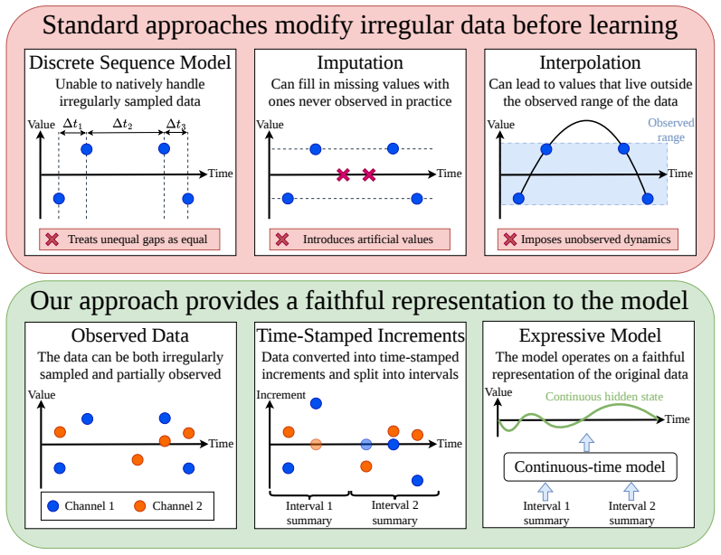
- Log-NCDEs become insensitive to the particular choice of interpolation or imputation used to reconstruct paths from discrete observations.
- The model can produce interval-level summaries directly from raw increments without first filling in values between observation times.
- Computation can proceed online because log-signatures are composed incrementally over successive query intervals.
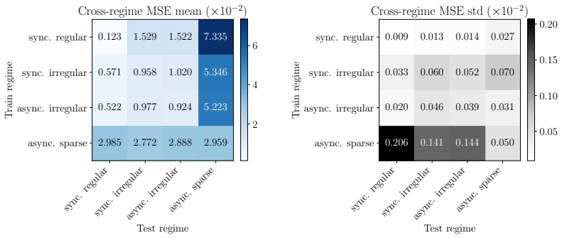
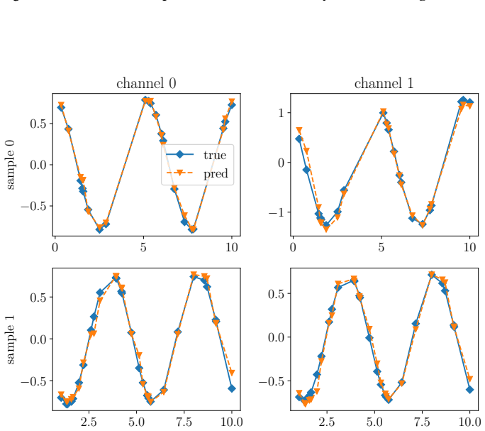
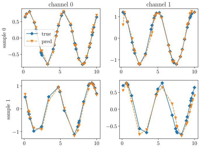
- The representation remains accurate and robust when tested on both synthetic controlled dynamics and real-world time-series datasets with irregular and sparse sampling.
Where Pith is reading between the lines
- The same transfer principle could be used to design faithful embeddings for other continuous-time architectures that currently rely on path reconstruction.
- In domains with streaming sensor data, the online property might allow models to update predictions as soon as new observations arrive without re-processing the entire history.
- One could explore whether relaxing injectivity while preserving continuity still yields useful approximation guarantees in practice.
Load-bearing premise
The mapping that turns sequences of discrete observations into the model's continuous input path must be both continuous and injective.
What would settle it
A counter-example where a continuous but non-injective embedding is used and the resulting Log-NCDE fails to approximate functions that the underlying model can approximate on the input space, or an empirical test on irregular data where the proposed embedding performs no better than standard interpolation methods.
Figures
read the original abstract
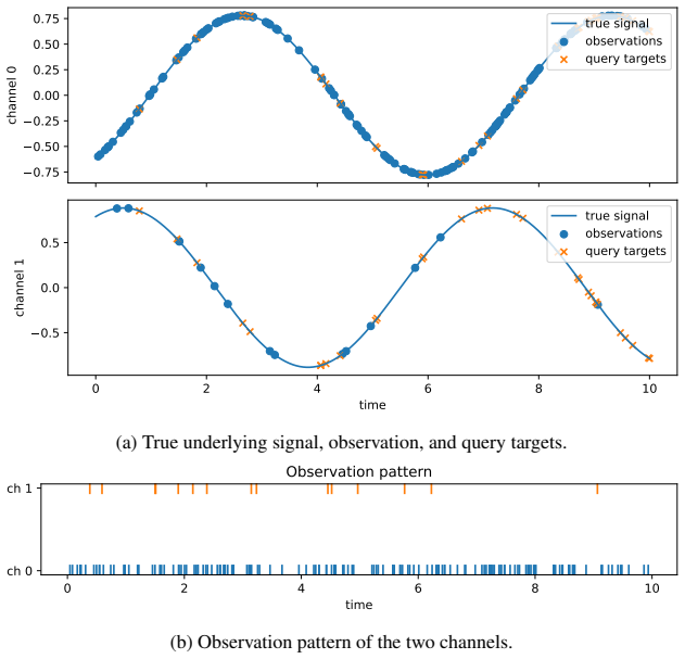
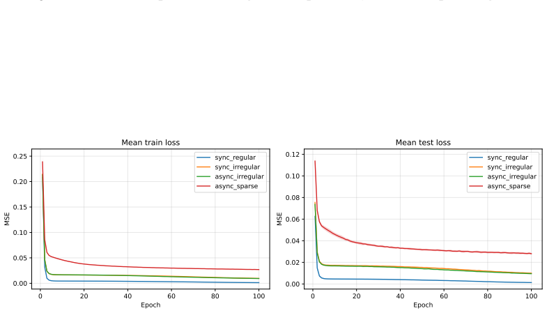
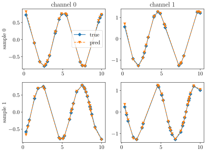
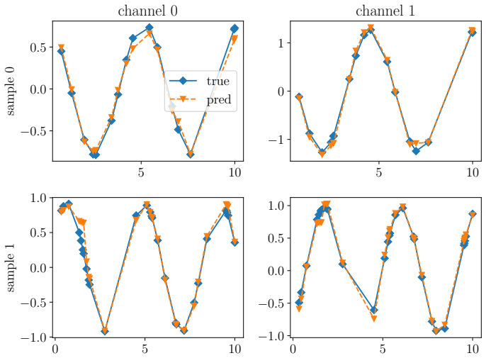
Continuous-time models are a natural choice for irregular and asynchronous data. A central design choice is how to embed discrete observations into continuous time. Interpolation- and imputation-based embeddings reconstruct a continuous observation path, making the model sensitive to the choice of reconstruction. We show that this reconstruction step is unnecessary; under mild conditions, compact-set universality on the model input space transfers to the data space whenever the embedding from data to input is continuous and injective. Guided by this result, and building on the rectilinear control path for Neural Controlled Differential Equations (NCDEs), we introduce a continuous and injective embedding for Log-NCDEs, a universal class of continuous-time models. Our approach records observations as increments and composes them over arbitrary query intervals to directly form log-signatures. This provides interval-level summaries without first interpolating the observed variables, while supporting online computation. Experiments on synthetic controlled dynamics and real-world time-series datasets show that the representation is accurate, efficient, and robust to irregular, asynchronous, and sparse observations.
Editorial analysis
A structured set of objections, weighed in public.
Referee Report
Summary. The paper claims that under mild conditions, compact-set universality on the model input space transfers to the data space whenever the embedding from data to input is continuous and injective. Guided by this, the authors introduce a continuous injective embedding for Log-NCDEs based on rectilinear control paths and log-signatures of observation increments, enabling online interval-level summaries without interpolation. Experiments on synthetic controlled dynamics and real-world time-series datasets are said to show accuracy, efficiency, and robustness to irregular, asynchronous, and sparse observations.
Significance. If the universality transfer result holds with the stated conditions, the work would supply a principled alternative to interpolation-based embeddings in continuous-time models, with direct benefits for online processing of irregular data. The focus on log-signature increments as interval summaries is a concrete technical contribution.
major comments (1)
- [Abstract] Abstract (central claim): the statement that compact-set universality transfers whenever the embedding is continuous and injective (under mild conditions) requires the mild conditions to guarantee that the inverse is continuous on the image of the embedding. Without a continuous inverse, functions of the form h ∘ φ need not be dense in C(K) for compact K in data space. The manuscript should state the mild conditions explicitly and verify they yield a topological embedding.
minor comments (1)
- The abstract references experimental results on synthetic and real-world datasets but provides no quantitative metrics, baselines, or controls; adding one or two key performance numbers would improve readability.
Simulated Author's Rebuttal
We thank the referee for the constructive comment on the central claim. We agree that the abstract requires clarification on the precise conditions and will revise accordingly to ensure the statement is accurate.
read point-by-point responses
-
Referee: [Abstract] Abstract (central claim): the statement that compact-set universality on the model input space transfers to the data space whenever the embedding from data to input is continuous and injective (under mild conditions) requires the mild conditions to guarantee that the inverse is continuous on the image of the embedding. Without a continuous inverse, functions of the form h ∘ φ need not be dense in C(K) for compact K in data space. The manuscript should state the mild conditions explicitly and verify they yield a topological embedding.
Authors: We appreciate this observation. The paper's main theorem (Section 3) states the universality transfer result under the assumption that the embedding is a topological embedding, which explicitly includes continuity of the inverse on the image. The phrase 'mild conditions' in the abstract is intended to refer to those ensuring the embedding property, but we acknowledge the summary is imprecise. In revision we will (i) restate the abstract to specify that the embedding must be a topological embedding and (ii) add a short remark or appendix verification confirming that the rectilinear log-signature construction satisfies the embedding conditions on the relevant compact sets of observation sequences. revision: yes
Circularity Check
No circularity: universality transfer is a general topological claim independent of paper inputs
full rationale
The paper's core claim is that compact-set universality transfers from model input space to data space whenever the embedding φ: data space → input space is continuous and injective (under mild conditions). This is stated as a general property of such maps rather than a derivation that reduces to its own fitted quantities or definitions by construction. No equations, parameters, or predictions in the provided abstract or description involve fitting a quantity to data and then renaming a related output as a 'prediction.' The new Log-NCDE embedding is motivated by the result but does not enter the statement of the transfer theorem itself. No self-citation load-bearing steps, uniqueness theorems imported from prior author work, or ansatzes smuggled via citation are present. The derivation chain is therefore self-contained against external mathematical benchmarks.
Axiom & Free-Parameter Ledger
axioms (1)
- domain assumption Compact-set universality transfers to data space under continuous and injective embedding
Reference graph
Works this paper leans on
-
[1]
ISSN 0899-7667. doi: 10.1162/neco.1997.9.8.1735. URL https://doi.org/10.1162/neco.1997. 9.8.1735. Christian Holberg and Cristopher Salvi. Exact gradients for stochastic spiking neural networks driven by rough signals. InProceedings of the 38th Conference on Neural Information Processing Systems (NeurIPS), 2024. Blanka Horvath, Maud Lemercier, Chong Liu, T...
-
[2]
URLhttps://doi.org/10.1137/23M161077X
doi: 10.1137/23M161077X. URLhttps://doi.org/10.1137/23M161077X. Sheo Yon Jhin, Jaehoon Lee, Minju Jo, Seungji Kook, Jinsung Jeon, Jihyeon Hyeong, Jayoung Kim, and Noseong Park. EXIT: Extrapolation and interpolation-based neural controlled differential equations for time-series classification and forecasting. InProceedings of the ACM Web Conference 2022, W...
-
[3]
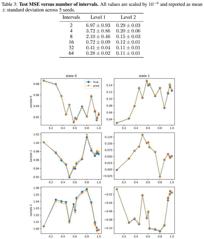
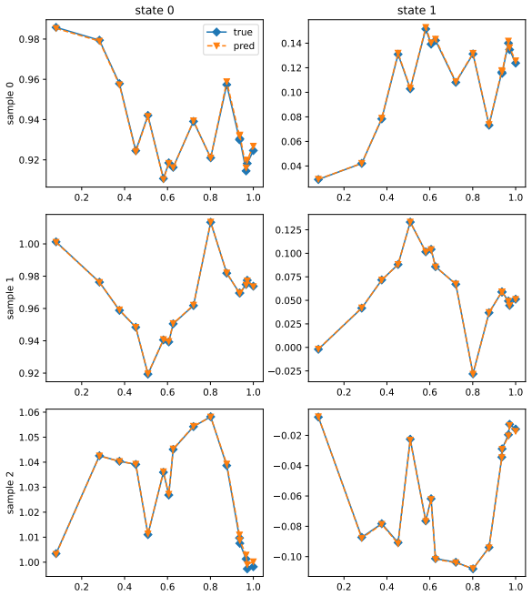
The same partition is used for all samples within a run
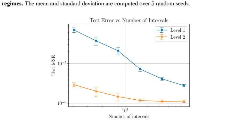
After rescaling by2048, this gives a random partition 0 =q 0 < q1 <· · ·< q m = 1. The same partition is used for all samples within a run. The target associated with interval [qk, qk+1) is the simulated state at the right endpoint, yk =X(q k+1)∈R 2. Although the model predicts endpoint values on a query grid that is separate from the fine input grid, the...
2048
discussion (0)
Sign in with ORCID, Apple, or X to comment. Anyone can read and Pith papers without signing in.