Flow map learning in nonlinear vector autoregressive models: influence of the feature-library structure on the training error
Pith reviewed 2026-06-28 23:17 UTC · model grok-4.3
The pith
The training error of nonlinear vector autoregressive models scales with time resolution according to laws set by whether the feature library exactly represents the early coefficients in the flow map expansion.
A machine-rendered reading of the paper's core claim, the machinery that carries it, and where it could break.
Core claim
The training error as a function of time resolution follows characteristic (pre-)asymptotic scaling laws that depend on whether the feature library can represent the early Lie-series coefficients of the flow map exactly or merely approximately. For dynamical systems governed by polynomial vector fields, this is shown for monomial and Fourier feature libraries in NVAR models, revealing the dependence on temporal resolution, nonlinear degree, and number of delay terms.
What carries the argument
The feature library structure and its exact or approximate representation of early Lie-series coefficients of the flow map, which governs the scaling laws of the training error.
Load-bearing premise
The dynamical systems under consideration are governed by polynomial vector fields.
What would settle it
An experiment that computes training errors for successively finer time resolutions in a polynomial vector field system and checks whether the error follows the predicted scaling for exact versus approximate library representations.
Figures
read the original abstract
Time series forecasting often requires learning nonlinear and time-delayed dependencies. A paradigmatic class of forecasting models are nonlinear vector autoregressive processes (NVAR), also known as next-generation reservoir computers (NG-RCs). These models approximate the Koopman operator on the space spanned by their explicit feature library. We consider the identifiability problem for learning Markovian nonlinear dynamical systems and show that the training error as a function of time resolution follows characteristic (pre-)asymptotic scaling laws. These laws depend on whether the feature library can represent the early Lie-series coefficients of the flow map (propagator) exactly or merely approximately. For dynamical systems governed by polynomial vector fields, we demonstrate the mechanism for NVAR/NG-RC models with monomial and Fourier feature libraries. We determine the dependence of the training error on the temporal resolution, the involved nonlinear degree, and the number of delay terms. While delay terms reduce the optimal one-step training error, they improve long-horizon forecasts only when the library provides sufficient nonlinearity. Thus, small training error coexists with weak generalization as the model class is mismatched to the true data-generating process. Numerical experiments on various chaotic dynamical systems confirm the theoretical predictions.
Editorial analysis
A structured set of objections, weighed in public.
Referee Report
Summary. The paper examines the identifiability problem in learning Markovian nonlinear dynamical systems via nonlinear vector autoregressive (NVAR/NG-RC) models, which approximate the Koopman operator using an explicit feature library. It derives that the training error as a function of time resolution obeys characteristic (pre-)asymptotic scaling laws determined by whether the library exactly or approximately represents the early Lie-series coefficients of the flow map. The analysis is restricted to polynomial vector fields and demonstrated explicitly for monomial and Fourier libraries, including the dependence of error on temporal resolution, nonlinear degree, and delay count. The work also shows that delay terms reduce optimal one-step training error but improve long-horizon forecasts only with sufficient nonlinearity in the library, and confirms the scaling predictions via numerical experiments on chaotic systems.
Significance. If the scaling laws and their dependence on exact versus approximate representation hold, the result supplies a concrete mechanism explaining why small training error can coexist with poor generalization when the model class mismatches the data-generating process. It clarifies the interplay between temporal resolution, library structure, and delay embedding in these Koopman-based forecasters, offering practical guidance for library design. The restriction to polynomial vector fields with explicit Lie-series termination, combined with numerical confirmation on standard chaotic benchmarks, constitutes a clear, falsifiable contribution within its stated scope.
minor comments (3)
- The abstract and introduction state the restriction to polynomial vector fields clearly, but §2 or the methods section should include an explicit remark that the exact-vs-approximate distinction and resulting scalings do not automatically extend to non-polynomial fields where the Lie series is infinite; this would prevent misreading by readers focused on general nonlinear systems.
- Figure captions for the numerical experiments should state the precise values of time step Δt, library degree, and number of delays used in each panel so that the reported scaling exponents can be directly compared to the derived expressions without consulting the main text.
- Notation for the Lie-series coefficients and the feature-library projection operator is introduced without a consolidated table; adding a short notation table would improve readability when the scaling arguments are revisited in the discussion of delay terms.
Simulated Author's Rebuttal
We thank the referee for their detailed summary of our manuscript and for the positive assessment of its contribution. The recommendation for minor revision is noted. No specific major comments were provided in the report, so we have no points to address point-by-point. We are prepared to incorporate any minor editorial changes requested by the editor.
Circularity Check
Derivation of scaling laws is self-contained; no circular reduction
full rationale
The paper derives (pre-)asymptotic scaling laws for training error versus time resolution from the structure of Lie-series coefficients of the flow map and whether monomial/Fourier libraries represent them exactly or approximately, restricted to polynomial vector fields. This is a first-principles analysis of model mismatch in NVAR/NG-RC setups, not a fit to data followed by a renamed prediction, nor a self-definitional loop, nor load-bearing self-citation. The abstract and description provide no equations or steps that reduce the claimed laws to inputs by construction; the result is independent of fitted parameters and externally falsifiable via the polynomial assumption and Lie expansion. No circularity patterns are exhibited.
Axiom & Free-Parameter Ledger
Reference graph
Works this paper leans on
-
[1]
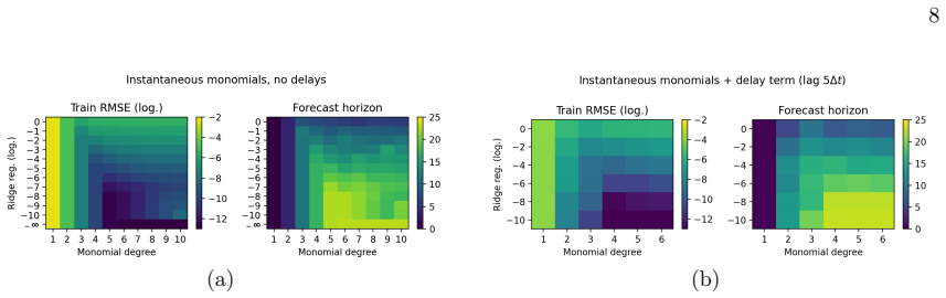
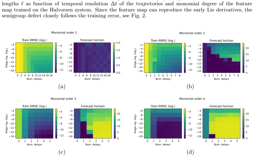
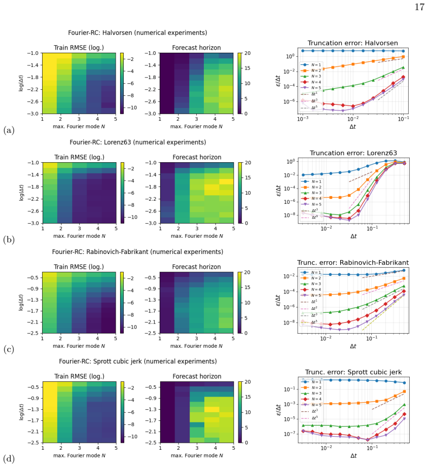
For raw monomial libraries, the RMS training error behaves approximately asε∼a(∆t) bM +ε floor(M, λ), with constantsa, b
Effect of monomial degree Figure 1 illustrates the training error and forecast horizon (obtained for the Halvorsen model) in dependence of the monomial degreeMof the feature library and the Ridge regularizationλ. For raw monomial libraries, the RMS training error behaves approximately asε∼a(∆t) bM +ε floor(M, λ), with constantsa, b. The first term is the ...
-
[2]
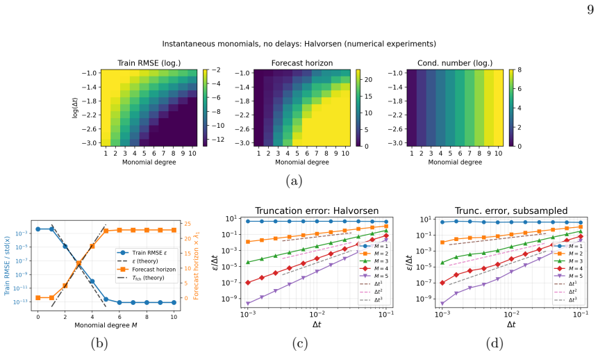
(3.8) until a floor is reached
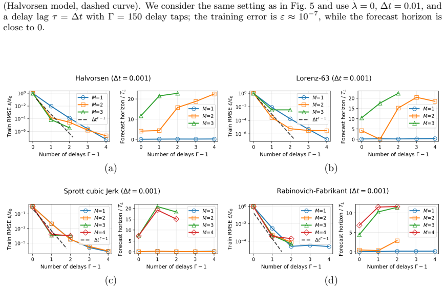
Effect of temporal resolution Figure 2(a,b) shows in more detail the behavior of the training error, following closely Eq. (3.8) until a floor is reached. The forecast horizonT fch grows according to Eq. (C12) with decreasingε. The saturation of the training error and forecast horizon is due to the integrator accuracy used to generate the trajectories and...
-
[3]
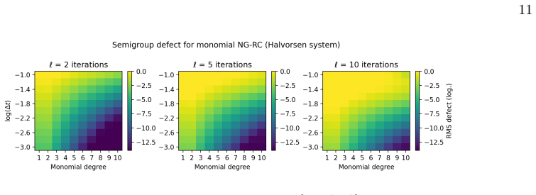
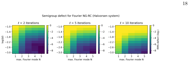
When the model can reproduce the early Lie derivatives of the true flow map, the error in the approximation in Eq
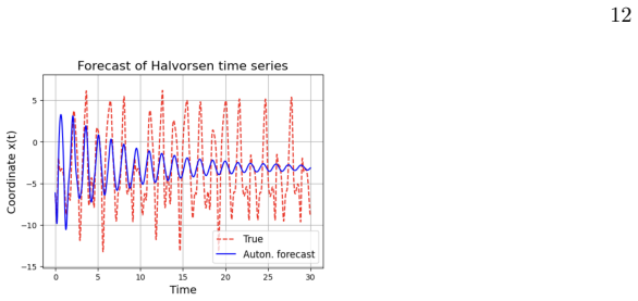
Semigroup consistency The semigroup consistency of a learned flow map bΦ∆t requires bΦℓ∆t ≈bΦℓ ∆t (4.7) wherebΦℓ ∆t =bΦ∆t ◦bΦ∆t ◦· · ·◦bΦ∆t (ℓtimes). When the model can reproduce the early Lie derivatives of the true flow map, the error in the approximation in Eq. (4.7) is proportional to the training error [see Eq. (A55)], Sm :=∥bΦℓ∆t −bΦℓ ∆t∥ ∼ε train.(...
-
[4]
Effect of delay terms Figure 5 demonstrates the influence of the number of time taps Γ on training error and forecast horizon at fixed monomial degreeM(Halvorsen model with ∆t= 0.01). When using only linear delays (M= 1), the NG-RC model becomes a linear autoregressive process and learns a harmonic approximation, often with a slowly decaying amplitude env...
-
[5]
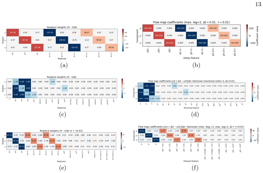
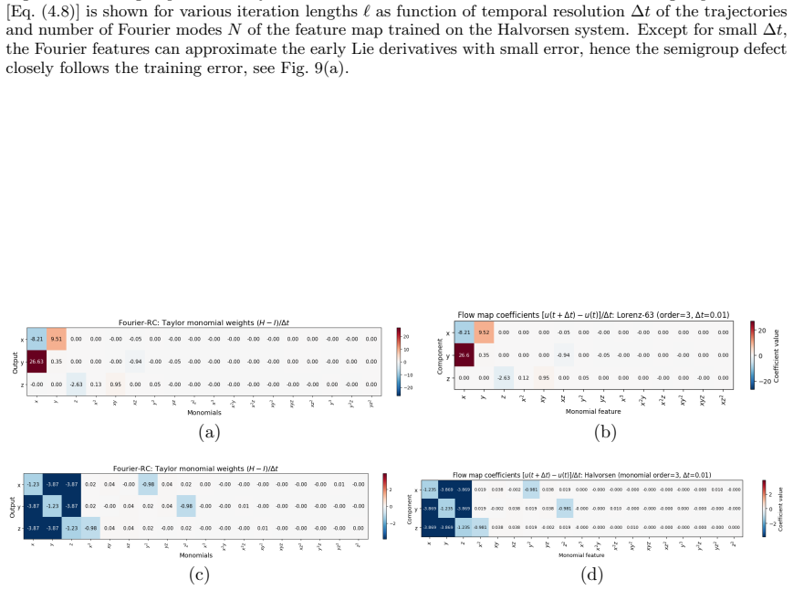
8, we compare the learned readout weights of a NG-RC trained on the Halvorsen system to the theoretical predictions in Section III B
Readout weights In Fig. 8, we compare the learned readout weights of a NG-RC trained on the Halvorsen system to the theoretical predictions in Section III B. A feature map consisting only of linear delay terms results in the generic weights of Eq. (3.17) (panels a,b). Conversely, if the feature map consists only of instantaneous monomials (panels c,d), th...
-
[6]
For a fixed target functionh∈L 2(µ;R d), the projectionPhis the best approximation tohamong all functions in V
A library-agnostic projection framework Given the feature mapg, the associated model class consists of all vector-valued functions that can be represented by a linear readout, V:= Hg(·) :H∈R d×n ⊂L 2(µ;R d).(A3) HereHis only a generic coefficient matrix parameterizing the elements ofV. For a fixed target functionh∈L 2(µ;R d), the projectionPhis the best a...
-
[7]
Asymptotic versus pre-asymptotic regimes If the vector field is not exactly representable by the feature library,f/∈V, thenε 1 >0 and the true asymptotic law is necessarily E(∆t) =ε 2 1∆t2 +O(∆t 3),(A14) Ifε 1 is much smaller thanε m for somem >1, different pre-asymptotic scalings are possible. Then, over a window of ∆tin which them-th term dominates in (...
-
[8]
Polynomial vector fields In order to make the previous discussion more concrete, consider the case whenfis polynomial of total degreep. In that case each Lie coefficientF m =L m−1 f fis again polynomial, with the degree bound degF m ≤1 +m(p−1), p >1.(A17) Hence the question reduces to how well the library reproduces polynomials of the degrees that are pro...
-
[9]
, N} d ,(A22) with base frequencyω 0
Fourier feature libraries We now consider flow map approximation with aN-frequency Fourier feature library: g(N)(x) = sin ω0 k·x ,cos ω0 k·x :k∈ {0, . . . , N} d ,(A22) with base frequencyω 0. Such a library can show extended pre-asymptotic error scaling before crossing over to the asymptotic law∝∆t 2. We assume the data reside in a box Ω⊂[−R, R] d, and d...
-
[10]
(A7) is the approximation-bias component of the usual bias–variance decomposition
Connection to bias–variance decomposition The projection error Eq. (A7) is the approximation-bias component of the usual bias–variance decomposition. In the increment-prediction setting of Section A 1, the target isF ∆t ∈L 2(µ;R d) and the model class is V={Hg(·) :H∈R d×n}.(A41) Leth ⋆ :=PF ∆t denote theL 2(µ)-orthogonal projection ofF ∆t ontoV. Then, for...
-
[11]
Consider now the difference betweenF [r] ∆t and the approximation of the true flow map by the feature library,PF ∆t ≈ ˆHg: in the same approximation-dominated regime as in Eq
Truncated flow-map error Since the exact expression for the flow mapF∆t is usually not available, consider its approximation to orderr F[r] ∆t(x) := Φ[r] ∆t(x)−x= rX m=1 ∆tm m! Fm(x),(A42) and define the difference to the true flow map asR [r] ∆t :=F ∆t −F [r] ∆t. Consider now the difference betweenF [r] ∆t and the approximation of the true flow map by th...
-
[12]
In the population limit, bΦh(x) :=x+PF h(x),(A51) theℓ-step semigroup defect is given by Sℓ(h)2 := bΦℓh −bΦℓ h 2 L2(µ) ,(A52) wherebΦℓ h denotesℓ-fold composition
Semigroup consistency The exact flow map satisfies the semigroup property [29] Φs+t = Φs ◦Φ t.(A50) This can be tested for the learned flow map bΦh, and we show that it essentially follows the same ∆t-scaling as the training error. In the population limit, bΦh(x) :=x+PF h(x),(A51) theℓ-step semigroup defect is given by Sℓ(h)2 := bΦℓh −bΦℓ h 2 L2(µ) ,(A52)...
-
[13]
, xd, ψ1,
Residual error and model bias Consider the flow map Φ ∆t(x), acting as x(t+ ∆t) = Φ ∆t x(t) ,(C1) and its approximation by a learned next-step map ˆx(t+ ∆t) = ˆH g ˆx(t) ,(C2) whereg= (x 1, . . . , xd, ψ1, . . . , ψm)∈R n is a reservoir vector. Consider the residual R(x)≡Φ ∆t(x)− ˆH g(x),(C3) 29 which we assume to be Lipschitz continuous with some constan...
-
[14]
Letx n+1 = Φ∆t(xn) be the true dynamics and ˆxn+1 = ˆH g(ˆxn) be the autonomous prediction obtained from the trained model
Error recurrence in autonomous forecasting We study the error evolution during autonomous forecasting. Letx n+1 = Φ∆t(xn) be the true dynamics and ˆxn+1 = ˆH g(ˆxn) be the autonomous prediction obtained from the trained model. Denoting the deviation between the two bye n =∥x n −ˆxn∥, we have en+1 =∥Φ ∆t(xn)− ˆH g(ˆxn)∥ ≤ ∥Φ ∆t(xn)−Φ ∆t(ˆxn)∥+∥Φ ∆t(ˆxn)− ˆ...
-
[15]
Lukoˇ seviˇ cius, A Practical Guide to Applying Echo State Networks, inNeural Networks: Tricks of the Trade, Vol
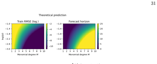
M. Lukoˇ seviˇ cius, A Practical Guide to Applying Echo State Networks, inNeural Networks: Tricks of the Trade, Vol. 7700, edited by G. Montavon, G. B. Orr, and K.-R. M¨ uller (Springer Berlin Heidelberg, Berlin, Heidelberg, 2012) pp. 659–686. 31 Figure 12. Theoretically predicted training errorε train ≃a∆t r∗+1 [Eq. (3.8)] and forecast horizonT fch ≃ ln(...
2012
-
[16]
Gilpin, Model scale versus domain knowledge in statistical forecasting of chaotic systems, Phys
W. Gilpin, Model scale versus domain knowledge in statistical forecasting of chaotic systems, Phys. Rev. Research5, 043252 (2023)
2023
-
[17]
M. Yan, C. Huang, P. Bienstman, P. Tino, W. Lin, and J. Sun, Emerging opportunities and challenges for the future of reservoir computing, Nature Communications15, 2056 (2024)
2056
-
[18]
Tanaka, T
G. Tanaka, T. Yamane, J. B. H´ eroux, R. Nakane, N. Kanazawa, S. Takeda, H. Numata, D. Nakano, and A. Hirose, Recent advances in physical reservoir computing: A review, Neural Networks115, 100 (2019)
2019
-
[19]
D. J. Gauthier, E. Bollt, A. Griffith, and W. A. S. Barbosa, Next generation reservoir computing, Nature Communications12, 5564 (2021)
2021
-
[20]
Shahi, F
S. Shahi, F. H. Fenton, and E. M. Cherry, Prediction of chaotic time series using recurrent neural net- works and reservoir computing techniques: A comparative study, Machine Learning with Applications 8, 100300 (2022)
2022
-
[21]
W. A. S. Barbosa and D. J. Gauthier, Learning spatiotemporal chaos using next-generation reservoir computing, Chaos: An Interdisciplinary Journal of Nonlinear Science32, 093137 (2022)
2022
- [22]
-
[23]
K¨ oglmayr and C
D. K¨ oglmayr and C. R¨ ath, Extrapolating tipping points and simulating non-stationary dynamics of complex systems using efficient machine learning, Scientific Reports14, 507 (2024)
2024
-
[24]
Brucke, S
K. Brucke, S. Schmitz, D. K¨ oglmayr, S. Baur, C. R¨ ath, E. Ansari, and P. Klement, Benchmarking reservoir computing for residential energy demand forecasting, Energy and Buildings314, 114236 (2024)
2024
-
[25]
C. Sch¨ otz, A. White, M. Gelbrecht, and N. Boers, Machine Learning for Predicting Chaotic Systems (2025), arXiv:2407.20158 [cs]
- [26]
-
[27]
I. J. Leontaritis and S. A. Billings, Input-output parametric models for non-linear systems Part I: Deterministic non-linear systems, International Journal of Control41, 303 (1985)
1985
-
[28]
Sparse Volterra and Polynomial Regression Models: Recoverability and Estimation
V. Kekatos and G. B. Giannakis, Sparse Volterra and Polynomial Regression Models: Recoverability and Estimation, IEEE Transactions on Signal Processing59, 5907 (2011), arXiv:1103.0769 [cs]
work page internal anchor Pith review Pith/arXiv arXiv 2011
-
[29]
S. A. Billings,Nonlinear System Identification: NARMAX Methods in the Time, Frequency, and Spatio-Temporal Domains(Wiley, 2013)
2013
-
[30]
Huang, Q.-Y
G.-B. Huang, Q.-Y. Zhu, and C.-K. Siew, Extreme learning machine: Theory and applications, Neu- rocomputing Neural Networks,70, 489 (2006)
2006
-
[31]
van Heeswijk, Y
M. van Heeswijk, Y. Miche, T. Lindh-Knuutila, P. A. J. Hilbers, T. Honkela, E. Oja, and A. Lendasse, Adaptive Ensemble Models of Extreme Learning Machines for Time Series Prediction, inArtificial Neural Networks – ICANN 2009, edited by C. Alippi, M. Polycarpou, C. Panayiotou, and G. Ellinas 32 (Springer, Berlin, Heidelberg, 2009) pp. 305–314
2009
-
[32]
Huang, D
G.-B. Huang, D. H. Wang, and Y. Lan, Extreme learning machines: A survey, International Journal of Machine Learning and Cybernetics2, 107 (2011)
2011
-
[33]
J. B. Butcher, D. Verstraeten, B. Schrauwen, C. R. Day, and P. W. Haycock, Reservoir computing and extreme learning machines for non-linear time-series data analysis, Neural Networks38, 76 (2013)
2013
-
[34]
Rahimi and B
A. Rahimi and B. Recht, Random Features for Large-Scale Kernel Machines, inAdvances in Neural Information Processing Systems, Vol. 20 (Curran Associates, Inc., 2007)
2007
-
[35]
M. O. Williams, I. G. Kevrekidis, and C. W. Rowley, A Data–Driven Approximation of the Koopman Operator: Extending Dynamic Mode Decomposition, Journal of Nonlinear Science25, 1307 (2015)
2015
-
[36]
S. L. Brunton and J. N. Kutz,Data-Driven Science and Engineering: Machine Learning, Dynamical Systems, and Control(Cambridge University Press, Cambridge, 2019)
2019
-
[37]
J. H. Tu, C. W. Rowley, D. M. Luchtenburg, S. L. Brunton, and J. N. Kutz, On Dynamic Mode Decomposition: Theory and Applications, Journal of Computational Dynamics1, 391 (2014), arXiv:1312.0041 [math]
work page internal anchor Pith review Pith/arXiv arXiv 2014
-
[38]
K. K. Chen, J. H. Tu, and C. W. Rowley, Variants of Dynamic Mode Decomposition: Boundary Condition, Koopman, and Fourier Analyses, Journal of Nonlinear Science22, 887 (2012)
2012
-
[39]
J. N. Kutz, S. L. Brunton, B. W. Brunton, and J. L. Proctor,Dynamic Mode Decomposition: Data-Driven Modeling of Complex Systems(SIAM-Society for Industrial and Applied Mathematics, Philadelphia, PA, USA, 2016)
2016
-
[40]
Korda and I
M. Korda and I. Mezi´ c, On Convergence of Extended Dynamic Mode Decomposition to the Koopman Operator, Journal of Nonlinear Science28, 687 (2018)
2018
-
[41]
Mezic, Koopman Operator, Geometry, and Learning (2020), arXiv:2010.05377 [math]
I. Mezic, Koopman Operator, Geometry, and Learning (2020), arXiv:2010.05377 [math]
-
[42]
Surana, Koopman Operator Framework for Time Series Modeling and Analysis, Journal of Non- linear Science30, 1973 (2020)
A. Surana, Koopman Operator Framework for Time Series Modeling and Analysis, Journal of Non- linear Science30, 1973 (2020)
1973
-
[43]
S. L. Brunton, M. Budiˇ si´ c, E. Kaiser, and J. N. Kutz, Modern Koopman Theory for Dynamical Systems, SIAM Review64, 229 (2022)
2022
-
[44]
Koopman-based lifting techniques for nonlinear systems identification
A. Mauroy and J. Goncalves, Koopman-based lifting techniques for nonlinear systems identification (2019), arXiv:1709.02003 [math]
work page internal anchor Pith review Pith/arXiv arXiv 2019
-
[45]
P. Bevanda, S. Sosnowski, and S. Hirche, Koopman Operator Dynamical Models: Learning, Analysis and Control, Annual Reviews in Control52, 197 (2021), arXiv:2102.02522 [eess]
-
[46]
S. E. Otto and C. W. Rowley, Koopman Operators for Estimation and Control of Dynamical Systems, Annual Review of Control, Robotics, and Autonomous Systems4, 59 (2021)
2021
-
[47]
Ghosh and M
R. Ghosh and M. Mcafee, Koopman operator theory and dynamic mode decomposition in data-driven science and engineering: A comprehensive review, Mathematical Modelling and Numerical Simulation with Applications4, 562 (2024)
2024
-
[48]
L. Shi, M. Haseli, G. Mamakoukas, D. Bruder, I. Abraham, T. Murphey, J. Cort´ es, and K. Karydis, Koopman Operators in Robot Learning, IEEE Transactions on Robotics42, 1088 (2026)
2026
-
[49]
Kowalski and W.-H
K. Kowalski and W.-H. Steeb,Nonlinear Dynamical Systems And Carleman Linearization(World Scientific, 1991)
1991
-
[50]
van Overschee and B
P. van Overschee and B. L. de Moor,Subspace Identification for Linear Systems: Theory — Imple- mentation — Applications(Springer, Boston, 1996)
1996
-
[51]
Ljung,System Identification: Theory for the User(Pearson, Upper Saddle River, NJ, 1999)
L. Ljung,System Identification: Theory for the User(Pearson, Upper Saddle River, NJ, 1999)
1999
-
[52]
S. L. Brunton, J. L. Proctor, and J. N. Kutz, Discovering governing equations from data by sparse identification of nonlinear dynamical systems, Proceedings of the National Academy of Sciences113, 3932 (2016)
2016
-
[53]
R. Iten, T. Metger, H. Wilming, L. del Rio, and R. Renner, Discovering Physical Concepts with Neural Networks, Phys. Rev. Lett.124, 010508 (2020)
2020
-
[54]
Z. Lai, C. Mylonas, S. Nagarajaiah, and E. Chatzi, Structural identification with physics-informed neural ordinary differential equations, Journal of Sound and Vibration508, 116196 (2021)
2021
-
[55]
C. Fronk and L. Petzold, Interpretable Polynomial Neural Ordinary Differential Equations, Chaos: An Interdisciplinary Journal of Nonlinear Science33, 043101 (2023), arXiv:2208.05072 [cs]
-
[56]
V. Churchill and D. Xiu, Flow Map Learning for Unknown Dynamical Systems: Overview, Imple- mentation, and Benchmarks (2023), arXiv:2307.11013 [cs]. 33
-
[57]
J. Chen and K. Wu, Deep-OSG: Deep Learning of Operators in Semigroup (2023), arXiv:2302.03358 [cs]
-
[58]
Yu and R
R. Yu and R. Wang, Learning dynamical systems from data: An introduction to physics-guided deep learning, Proceedings of the National Academy of Sciences121, e2311808121 (2024)
2024
-
[59]
Koltai and P
P. Koltai and P. Kunde, A Koopman–Takens Theorem: Linear Least Squares Prediction of Nonlinear Time Series, Communications in Mathematical Physics405, 120 (2024)
2024
-
[60]
Zhang and E
C. Zhang and E. Zuazua, A quantitative analysis of Koopman operator methods for system identifi- cation and predictions, Comptes Rendus. M´ ecanique351, 721 (2024)
2024
- [61]
-
[62]
C.-B. Sch¨ onlieb and Z. Shumaylov, Data-driven approaches to inverse problems (2025), arXiv:2506.11732 [math]
-
[63]
Z. Shumaylov, P. Zaika, P. Scholl, G. Kutyniok, L. Horesh, and C.-B. Sch¨ onlieb, When is a System Discoverable from Data? Discovery Requires Chaos (2025), arXiv:2511.08860 [math]
-
[64]
H. Parikh, Why are there many equally good models? An Anatomy of the Rashomon Effect (2026), arXiv:2601.06730 [cs]
-
[65]
Roeder, L
G. Roeder, L. Metz, and D. Kingma, On Linear Identifiability of Learned Representations, inPro- ceedings of the 38th International Conference on Machine Learning(PMLR, 2021) pp. 9030–9039
2021
-
[66]
Gy¨ orgyi, First-order transition to perfect generalization in a neural network with binary synapses, Phys
G. Gy¨ orgyi, First-order transition to perfect generalization in a neural network with binary synapses, Phys. Rev. A41, 7097 (1990)
1990
-
[67]
H. S. Seung, Statistical mechanics of learning from examples, Phys. Rev. A45, 6056 (1992)
1992
-
[68]
T. L. H. Watkin, The statistical mechanics of learning a rule, Reviews of Modern Physics65, 499 (1993)
1993
- [69]
-
[70]
G. E. Karniadakis, I. G. Kevrekidis, L. Lu, P. Perdikaris, S. Wang, and L. Yang, Physics-informed machine learning, Nature Reviews Physics3, 422 (2021)
2021
- [71]
- [72]
-
[73]
B. Russo and M. P. Laiu, Convergence of weak-SINDy Surrogate Models (2024), arXiv:2209.15573 [math]
-
[74]
Pecile, N
A. Pecile, N. Demo, M. Tezzele, G. Rozza, and D. Breda, Data-driven discovery of delay differential equations with discrete delays, Journal of Computational and Applied Mathematics461, 116439 (2025)
2025
-
[75]
Zhang and S
Y. Zhang and S. P. Cornelius, Catch-22s of reservoir computing, Phys. Rev. Research5, 033213 (2023)
2023
- [76]
- [77]
-
[78]
S. Liu, J. Xiao, Z. Yan, and J. Gao, Noise resistance of next-generation reservoir computing: A comparative study with high-order correlation computation, Nonlinear Dynamics111, 14295 (2023)
2023
- [79]
-
[80]
Kay and S
S. Kay and S. Marple, Spectrum analysis—A modern perspective, Proceedings of the IEEE69, 1380 (1981)
1981
discussion (0)
Sign in with ORCID, Apple, or X to comment. Anyone can read and Pith papers without signing in.