Giving Sensors a Voice: Multimodal JEPA for Semantic Time-Series Embeddings
Pith reviewed 2026-06-28 23:07 UTC · model grok-4.3
The pith
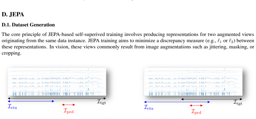
Textual descriptions of sensor channels combined with joint embedding prediction let a transformer learn time-series embeddings that perform strongly on multiple tasks via linear probes alone.
A machine-rendered reading of the paper's core claim, the machinery that carries it, and where it could break.
Core claim
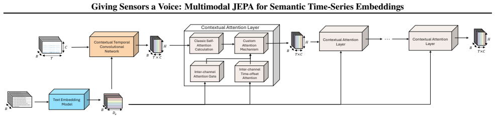
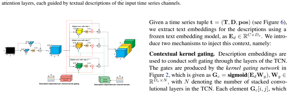
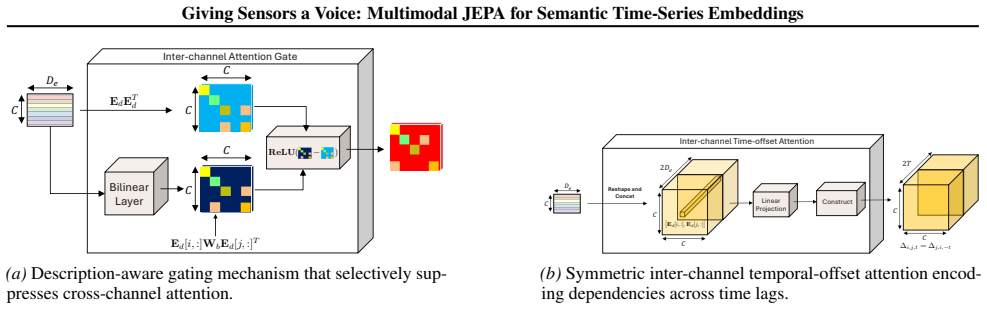
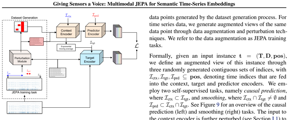
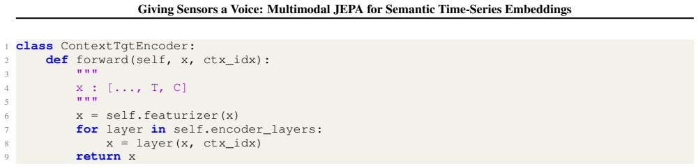
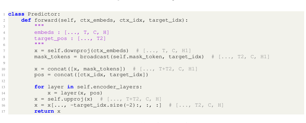
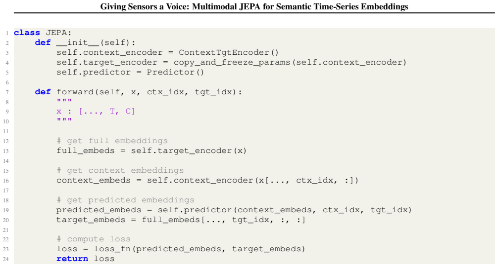
CHARM incorporates channel-level textual descriptions into a Transformer encoder equivariant to channel order. It is trained with a Joint Embedding Predictive Architecture (JEPA) and a novel loss promoting informative, temporally stable embeddings. Latent-space prediction encourages robustness to sensor noise while description-aware gating provides interpretability through learned inter-channel relationships. Across anomaly detection, classification, and short- and long-term forecasting, the learned embeddings achieve strong performance using only a linear probe. Performance is driven primarily by the JEPA objective and conditioning architecture, with text descriptions serving as channel ide
What carries the argument
CHARM, the Channel-Aware Representation Model: a channel-order-equivariant transformer that uses description-aware gating and is trained by joint embedding prediction in latent space.
If this is right
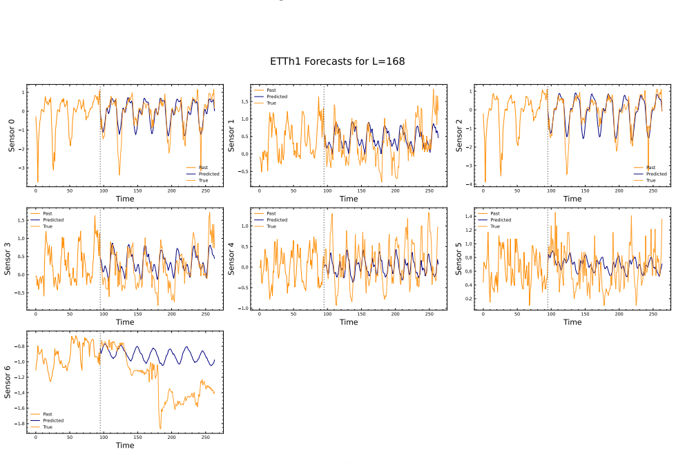
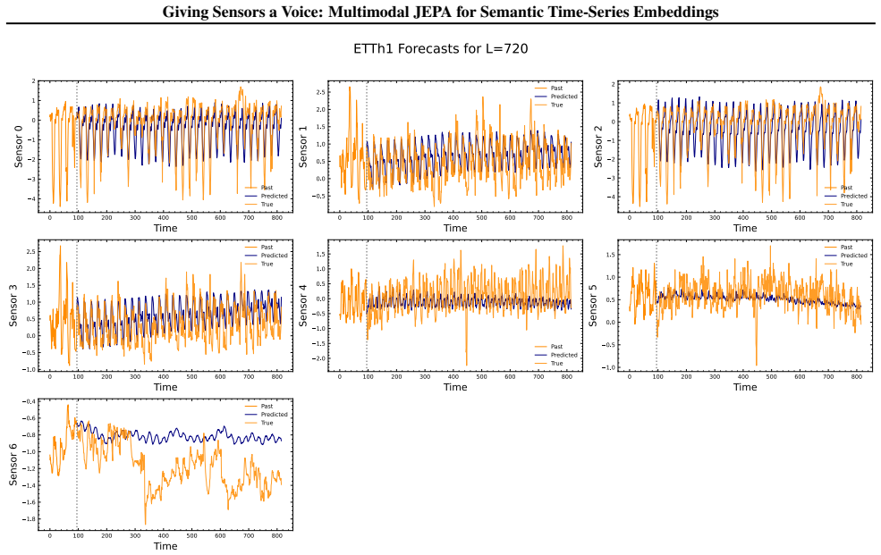
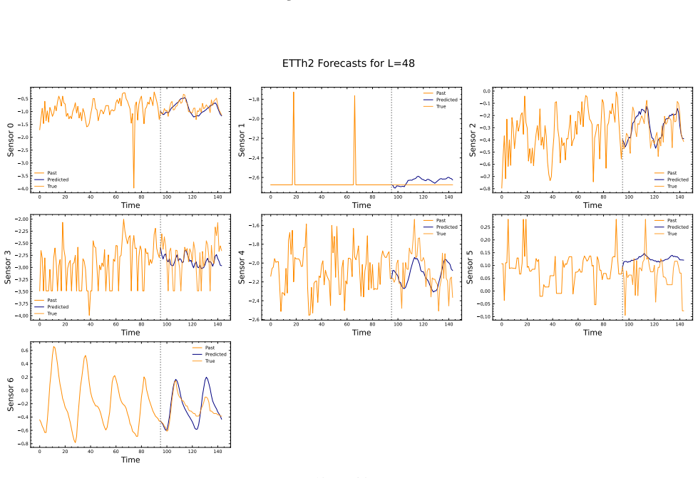
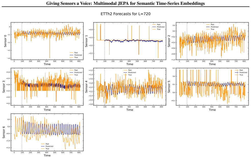
- The embeddings support anomaly detection, classification, short-term forecasting and long-term forecasting when paired with a linear probe.
- Performance is driven mainly by the joint embedding prediction objective and the conditioning architecture.
- Text descriptions function chiefly as channel identifiers that support generalization across different datasets.
- Latent-space prediction builds robustness to sensor noise.
- Description-aware gating learns interpretable inter-channel relationships.
Where Pith is reading between the lines
- Standardized channel descriptions could let the same embeddings transfer to entirely new sensor configurations without retraining.
- The same conditioning pattern might be applied to other data types where metadata can be expressed in short text.
- Because the embeddings already capture long-horizon structure, they could serve as drop-in features for control or planning loops that require future-state estimates.
- Pairing the embeddings with a language model might allow natural-language queries over raw sensor streams.
Load-bearing premise
The quality of the embeddings is produced by the joint embedding prediction objective together with description-aware gating rather than by dataset-specific fitting or choices made after training.
What would settle it
A controlled experiment in which a plain transformer without the JEPA loss or the text-based gating reaches comparable linear-probe accuracy on the same anomaly detection, classification, and forecasting benchmarks would falsify the claim that those two components drive performance.
Figures
read the original abstract
Transformer-based architectures have advanced sequence modeling in language and vision, yet general-purpose representation learning for heterogeneous multivariate time series remains underexplored. We introduce CHARM (Channel-Aware Representation Model), which incorporates channel-level textual descriptions into a Transformer encoder equivariant to channel order. CHARM is trained with a Joint Embedding Predictive Architecture (JEPA) and a novel loss promoting informative, temporally stable embeddings; latent-space prediction encourages robustness to sensor noise while description-aware gating provides interpretability through learned inter-channel relationships. Across anomaly detection, classification, and short- and long-term forecasting, the learned embeddings achieve strong performance using only a linear probe. Performance is driven primarily by the JEPA objective and conditioning architecture, with text descriptions serving as channel identifiers for cross-dataset generalization.
Editorial analysis
A structured set of objections, weighed in public.
Referee Report
Summary. The paper introduces CHARM (Channel-Aware Representation Model), a Transformer encoder for heterogeneous multivariate time series made equivariant to channel order via incorporation of channel-level textual descriptions. The model is trained with a Joint Embedding Predictive Architecture (JEPA) objective plus a novel loss promoting informative and temporally stable embeddings; latent prediction is intended to confer robustness to sensor noise while description-aware gating supplies interpretability. Embeddings are evaluated on anomaly detection, classification, and short- and long-term forecasting tasks using only linear probes, with the central claim that performance is driven primarily by the JEPA objective and conditioning architecture rather than dataset-specific fitting, and that text descriptions function as channel identifiers enabling cross-dataset generalization.
Significance. If the experimental controls confirm that the reported gains are attributable to the JEPA training objective and multimodal conditioning rather than post-hoc fitting or evaluation choices, the work would constitute a meaningful contribution to general-purpose time-series representation learning by demonstrating how JEPA-style latent prediction combined with textual channel conditioning can yield robust, interpretable embeddings across heterogeneous sensor datasets.
major comments (1)
- [Abstract and §4] Abstract and §4 (experimental claims): the assertion that 'performance is driven primarily by the JEPA objective and conditioning architecture' is load-bearing for the central contribution yet is not accompanied by the ablations or controls needed to rule out dataset-specific fitting or post-hoc evaluation artifacts; without these, the claim that text descriptions serve only as channel identifiers for generalization cannot be assessed.
minor comments (2)
- The abstract would benefit from naming the specific datasets and reporting at least one quantitative metric (e.g., AUC or MSE improvement) to allow readers to gauge the strength of the 'strong performance' claim.
- [§3] Notation for the description-aware gating mechanism should be introduced with an equation or diagram in §3 to clarify how textual embeddings modulate the Transformer layers.
Simulated Author's Rebuttal
We thank the referee for highlighting the need for stronger controls to support the central claims. We will revise the manuscript to include the requested ablations and cross-dataset experiments.
read point-by-point responses
-
Referee: [Abstract and §4] Abstract and §4 (experimental claims): the assertion that 'performance is driven primarily by the JEPA objective and conditioning architecture' is load-bearing for the central contribution yet is not accompanied by the ablations or controls needed to rule out dataset-specific fitting or post-hoc evaluation artifacts; without these, the claim that text descriptions serve only as channel identifiers for generalization cannot be assessed.
Authors: We agree that the load-bearing claim requires explicit ablations to isolate the JEPA objective, channel conditioning, and text descriptions from potential dataset-specific fitting or evaluation artifacts. In the revised manuscript we will add: (1) ablation replacing the JEPA latent-prediction loss with standard reconstruction and contrastive baselines while keeping the architecture fixed; (2) ablation removing description-aware gating (replacing channel text with random or positional identifiers); (3) cross-dataset transfer experiments in which embeddings trained on one sensor collection are linearly probed on another to test whether text descriptions function as general channel identifiers. These controls will directly address concerns about post-hoc artifacts and will be reported in an expanded §4 with quantitative tables. revision: yes
Circularity Check
No significant circularity identified
full rationale
The provided abstract and context describe an empirical model (CHARM) trained via JEPA objective on time-series data, with performance evaluated via linear probes on downstream tasks. No derivation chain, equations, fitted parameters renamed as predictions, or self-citation load-bearing steps are present that would reduce any claimed result to its inputs by construction. The central claims rest on training objectives and empirical results rather than definitional equivalence or imported uniqueness theorems, making the work self-contained against external benchmarks.
Axiom & Free-Parameter Ledger
Reference graph
Works this paper leans on
-
[1]
URL https://openreview.net/pdf? id=UVF1AMBj9u. poster. Chen, M., Shen, L., Li, Z., Wang, X. J., Sun, J., and Liu, C. Visionts: Visual masked autoencoders are free-lunch zero-shot time series forecasters, 2025. URL https: //arxiv.org/abs/2408.17253. Chen, S., Gong, C., Li, J., Yang, J., Niu, G., and Sugiyama, M. Learning contrastive embedding in low-dimens...
-
[2]
URL https://doi.org/10.48550/ arXiv.2412.10925. Edwards, T. D. P., Alvey, J., Alsing, J., Nguyen, N. H., and Wandelt, B. D. Scaling-laws for large time-series mod- els, 2025. URL https://arxiv.org/abs/2405. 13867. Falcon, W. and The PyTorch Lightning team. PyTorch Light- ning, March 2019. URL https://github.com/ Lightning-AI/lightning. Fleming, P. J. and ...
-
[3]
The learning rate follows a linear warmup followed by a cosine decay
Optimization ScheduleWe use an AdamW optimizer to optimize our model. The learning rate follows a linear warmup followed by a cosine decay
-
[4]
Weight InitializationWe use a fixed N(0,0.02) initialization which is commonly used in pretraining large transformer models (OLMo et al., 2025)
2025
-
[5]
Weight Decay SchedulingWe use a cosine schedule for increasing the optimizer’s weight decay over the course of training which has been shown to be crucial for training stability
-
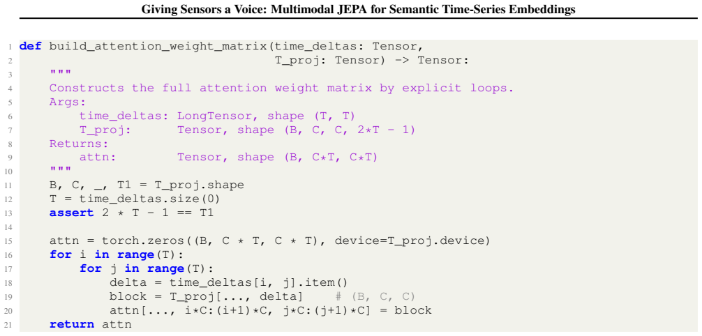
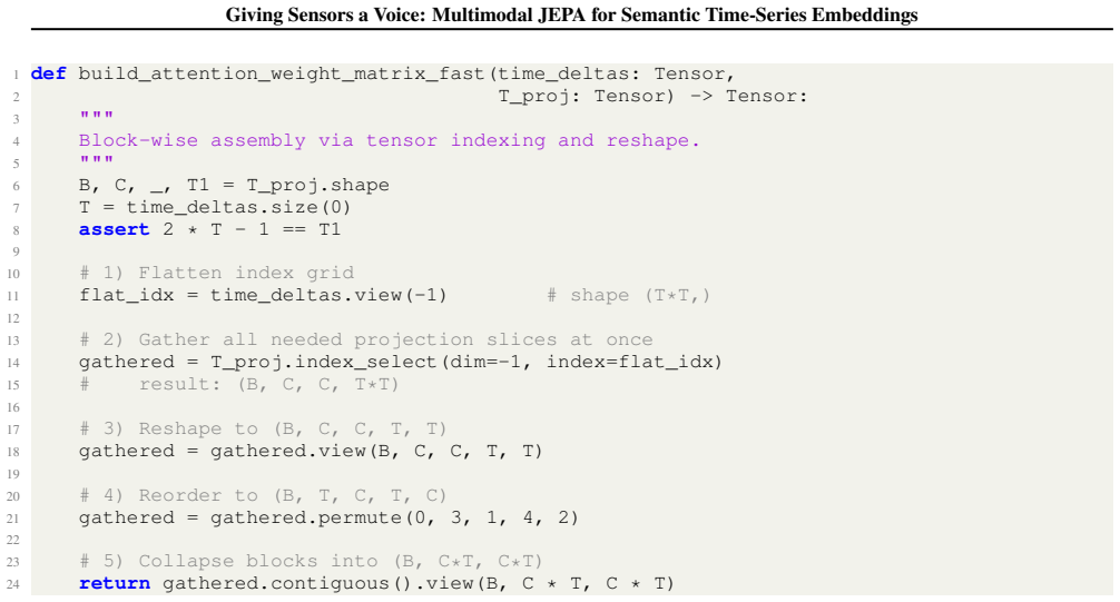
[6]
"" 4Block-wise assembly via tensor indexing and reshape. 5
EMA Schedule for Target EncoderWe use an exponentially moving average with a momentum schedule that is increased gradually over the course of training. The weight decay scheduling and EMA schedule are identical to IJEPA (Assran et al., 2023). Besides sweeping over a few learning rates, we perform no additional hyperparameter tuning on the rest of the hype...
2023
-
[7]
Time Series Classification Models:MiniRocket
-
[8]
Semantic Representation Learning Models :T-Rep,TS2Vec,T-Loss,TS-TCCetc
-
[9]
Reconstruction Based Representation Learning Models :MOMENT Given our limited compute availability, all baseline results reported in the results table are drawn from prior published work. We restrict our comparison to models with results on the majority of the UEA datasets, and therefore exclude models with incomplete or missing UEA coverage (e.g., UniTS)...
-
[10]
||xtest −ˆxtest|| lie outside the UCL limit
Then, for the reconstructed test data ˆxtest, we classify anomalies if the absolute values of the residuals, i.e. ||xtest −ˆxtest|| lie outside the UCL limit. This exact anomaly detection setup is commonly applied to all baseline models in the test suite. Downstream Setup.Similar to J.2.1, we rely on training a linear head to reconstruct“clean” training d...
2021
-
[11]
CHARM+NLH:A common non-linear prediction head is trained across all datasets, channels, and horizons, with the encoder kept frozen
-
[12]
CHARM+NLH FT:The full model (encoder + non-linear prediction head) is trained end-to-end, shared across datasets, channels, and horizons. Non-Linear Head (NLH)The head is designed to first mix information across both time and channels, then refine within each channel, and finally project to the forecasting horizon: • Transformer across time & channels (nh...
-
[13]
Z:R T×H →Z mean ∈R H 3.Last Time Step: The embedding from the last time step of each channel is taken as the representative embedding
Mean Pooling: The embeddings are averaged over the time dimension (but not across channels), yielding an H- dimensional representation per channel. Z:R T×H →Z mean ∈R H 3.Last Time Step: The embedding from the last time step of each channel is taken as the representative embedding. Z:R T×H →Z −1 ∈R H In addition, we experimented with: • Frozen Encoder + 2...
2024
-
[14]
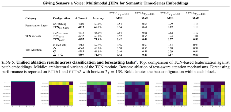
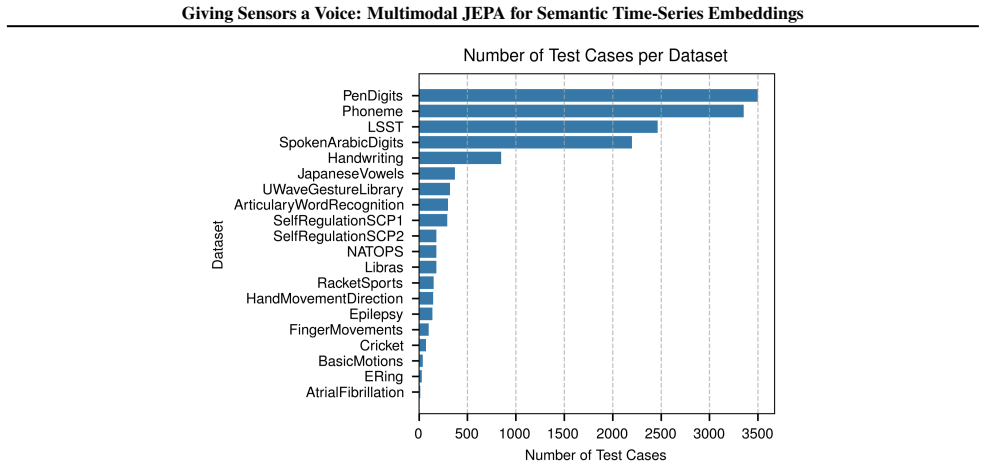
Total number of correct classifications for UEA
-
[15]
Average accuracy for UEA
-
[16]
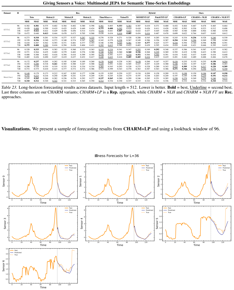
Mean Squared Error for ETTh1 (T f = 168)
-
[17]
Mean Absolute Error for ETTh1 (T f = 168)
-
[18]
Mean Squared Error for ETTh2 (T f = 168)
-
[19]
Classification Evaluations.The hyperparameters used for measuring classification performance are listed in Table 25
Mean Absolute Error for ETTh2 (T f = 168) For the ablation study, we train and probe the model with the following protocols: Pretraining.The base model is pretrained with a subset of datasets (UEA, ETTh, ETTm, Weather, Illness), for 50 epochs, with a learning rate of 5e-4. Classification Evaluations.The hyperparameters used for measuring classification pe...
-
[20]
These are obtained through either manual human annotation obtained by parsing the accompanying dataset metadata files, or are natively provided by the dataset provider
Annotated descriptions: manually curated sensor descriptions obtained from the official dataset metadata. These are obtained through either manual human annotation obtained by parsing the accompanying dataset metadata files, or are natively provided by the dataset provider
-
[21]
Noisy descriptions: high quality annotated descriptions, but with words dropped at random (with p= 0.2 ) during both training and evaluation
-
[22]
Ordinal descriptions: replace the annotated descriptions with structured, placeholder descriptions: [ Sensor1, Sensor2,Sensor3...] for all datasets. •(iv) Effect of text embedding model We investigate the usage of different embedding models to assess the effect on downstream performance. We use 1) nomic (Nussbaum et al., 2025), 2) minilm (Wang et al., 202...
discussion (0)
Sign in with ORCID, Apple, or X to comment. Anyone can read and Pith papers without signing in.