Tailoring Strictly Proper Scoring Rules for Downstream Tasks: An Application to Causal Inference
Pith reviewed 2026-06-28 11:19 UTC · model grok-4.3
The pith
A framework derives task-specific strictly proper scoring rules by matching curvature of the downstream error metric, yielding a closed-form loss for ATE estimation.
A machine-rendered reading of the paper's core claim, the machinery that carries it, and where it could break.
Core claim
The authors establish that strictly proper scoring rules can be obtained systematically by matching the local curvature of any chosen downstream error metric, and that the resulting rule for the IPW estimator of the Average Treatment Effect admits a closed-form expression whose optimization yields propensity scores that improve final ATE accuracy over likelihood-based training.
What carries the argument
The curvature-matching construction of task-specific strictly proper scoring rules; it aligns the second-order behavior of the scoring rule with the downstream IPW error so that its minimum corresponds to the probabilities that minimize that error.
If this is right
- The closed-form loss and probability mapping integrate directly with any differentiable or tree-based model for propensity estimation.
- Optimization under the tailored rule produces propensity scores that reduce both bias and variance in the final IPW ATE estimator.
- The same curvature-matching procedure applies to other downstream metrics by replacing the IPW error with the metric of interest.
- On standard causal inference benchmarks the method outperforms both likelihood training and covariate-balancing alternatives.
Where Pith is reading between the lines
- The same construction could be applied to other causal estimators such as the average treatment effect on the treated or to non-causal tasks whose error surfaces are known.
- End-to-end pipelines could back-propagate through the curvature-derived loss when the downstream metric itself depends on the model parameters.
- Empirical checks on data sets containing unmeasured confounding would test whether the curvature alignment remains beneficial outside the paper's simulation and benchmark settings.
Load-bearing premise
That matching the local curvature of the IPW error metric produces a strictly proper scoring rule whose optimization yields lower bias and variance in the ATE estimate than standard likelihood training.
What would settle it
On a benchmark dataset with known ground-truth ATE, train identical models with the derived loss versus log-loss and measure whether the mean squared error of the resulting ATE estimate is not smaller for the new loss.
Figures
read the original abstract
Probabilistic models are typically trained using task-agnostic objectives like log-loss, which can lead to significant errors in downstream estimation. This disconnect is especially critical in Inverse Probability Weighting (IPW) for causal inference, where propensity score errors near $0$ and $1$ often lead to high bias and variance. We propose a principled framework for deriving task-specific strictly proper scoring rules by matching the local curvature of the downstream error metric. We apply this to the Average Treatment Effect (ATE) estimation, deriving a closed-form loss and its corresponding canonical probability mapping that can be readily integrated with any model like a neural network or a gradient boosting algorithm. Extensive evaluations on causal inference benchmarks demonstrate that our tailored objective consistently outperforms standard likelihood-based and covariate-balancing approaches.
Editorial analysis
A structured set of objections, weighed in public.
Referee Report
Summary. The manuscript proposes a framework for deriving task-specific strictly proper scoring rules by matching the local curvature of a downstream error metric to the Hessian of the scoring rule. Applied to Average Treatment Effect (ATE) estimation via Inverse Probability Weighting (IPW), it derives a closed-form loss together with a canonical probability mapping that can be plugged into any probabilistic model (neural nets, gradient boosting). Extensive benchmark experiments are reported to show that the tailored objective yields lower bias and variance than standard log-loss or covariate-balancing baselines.
Significance. If the derived rule is provably strictly proper and the reported gains are reproducible, the work would provide a principled route to align training objectives with downstream causal estimators, addressing a known weakness of propensity-score models near the probability boundaries.
major comments (2)
- [§3] §3 (Curvature-matching derivation): The claim that the resulting functional is a strictly proper scoring rule rests on local Hessian agreement with the IPW error metric. Because the IPW variance term is non-convex in p near 0 and 1, local curvature matching does not automatically guarantee that the expected score is uniquely minimized at the true conditional probability for every distribution; an explicit proof that the derived loss belongs to the Bregman-divergence family or satisfies the global uniqueness condition is required.
- [§4] §4 (Closed-form loss and canonical mapping): The manuscript states that the derived loss remains strictly proper after the canonical probability mapping is applied. It is unclear whether the mapping preserves the strict properness property or merely approximates it; the relevant theorem or proposition should be stated with its assumptions and proof sketch.
minor comments (2)
- [Table 2] Table 2: the reported standard errors for the ATE estimates appear to be computed under the assumption that the propensity model is fixed; clarify whether they account for the joint estimation of the tailored loss.
- [Figure 3] Figure 3 caption: the legend does not distinguish the curves corresponding to the proposed loss from those of the baseline log-loss; add explicit labels.
Simulated Author's Rebuttal
We thank the referee for the careful and constructive review. The comments highlight important points regarding the theoretical guarantees of strict properness. We address each major comment below and will revise the manuscript to strengthen the presentation of the proofs.
read point-by-point responses
-
Referee: [§3] §3 (Curvature-matching derivation): The claim that the resulting functional is a strictly proper scoring rule rests on local Hessian agreement with the IPW error metric. Because the IPW variance term is non-convex in p near 0 and 1, local curvature matching does not automatically guarantee that the expected score is uniquely minimized at the true conditional probability for every distribution; an explicit proof that the derived loss belongs to the Bregman-divergence family or satisfies the global uniqueness condition is required.
Authors: We agree that local Hessian matching alone does not automatically imply global strict properness, particularly given the non-convexity of the IPW variance near the boundaries. The manuscript's derivation implicitly relies on the resulting functional being a Bregman divergence, but an explicit statement is indeed needed. In the revision we will add a new proposition (with proof) establishing that the derived scoring rule is generated by a strictly convex function whose Bregman divergence coincides with the local curvature of the IPW error metric; the proof will verify unique minimization at the true conditional probability for all distributions in the interior of the probability simplex and will explicitly address boundary behavior. revision: yes
-
Referee: [§4] §4 (Closed-form loss and canonical mapping): The manuscript states that the derived loss remains strictly proper after the canonical probability mapping is applied. It is unclear whether the mapping preserves the strict properness property or merely approximates it; the relevant theorem or proposition should be stated with its assumptions and proof sketch.
Authors: The canonical mapping is constructed to be a strictly increasing, differentiable bijection that preserves the unique minimizer of the expected score. We will add a dedicated theorem in §4 that states the precise assumptions (the mapping must be strictly increasing with derivative bounded away from zero at the boundaries) and provides a short proof sketch showing that composition with the mapping preserves membership in the Bregman-divergence family, thereby retaining strict properness. The theorem will also note that the mapping does not alter the location of the minimum. revision: yes
Circularity Check
No circularity; derivation is first-principles curvature matching
full rationale
The paper derives task-specific scoring rules from the explicit principle of matching local curvature (second derivative) of the downstream IPW error metric to the scoring rule's Hessian, then obtains a closed-form loss for ATE. This construction is independent of the final ATE estimate and does not reduce to a fit, self-definition, or self-citation chain. No load-bearing self-citations, fitted inputs renamed as predictions, or ansatzes smuggled via prior work appear in the provided text. The framework is therefore self-contained against external benchmarks; any question of whether local matching suffices for global strict properness is a correctness issue, not circularity.
Axiom & Free-Parameter Ledger
axioms (2)
- standard math Strictly proper scoring rules are minimized uniquely at the true conditional probabilities.
- domain assumption The downstream error metric for IPW/ATE has a local curvature that can be directly matched to produce an optimal scoring rule.
Reference graph
Works this paper leans on
-
[1]
ISSN 0025-1909. doi: 10.1287/mnsc.2018.3253. URL https://doi.org/10.1287/mnsc.2018. 3253. Blondel, M., Martins, A. F., and Niculae, V . Learning with fenchel-young losses.Journal of Machine Learning Research, 21(35):1–69, 2020. URL http://jmlr. org/papers/v21/19-021.html. Bruns-Smith, D. A. and Feller, A. Outcome assumptions and duality theory for balanci...
-
[2]
PMLR, 2022. URL https://proceedings. mlr.press/v162/chernozhukov22a.html. Crump, R. K., Hotz, V . J., Imbens, G. W., and Mitnik, O. A. Dealing with limited overlap in estimation of average treatment effects.Biometrika, 96(1):187–199, 01 2009. ISSN 0006-3444. doi: 10.1093/biomet/asn055. URL https://doi.org/10.1093/biomet/asn055. Dembczynski, K., Waegeman, ...
-
[3]
Donti, P., Amos, B., and Kolter, J
URL https://proceedings.mlr.press/ v244/deshpande24a.html. Donti, P., Amos, B., and Kolter, J. Z. Task-based end-to-end model learning in stochastic optimization. In Guyon, I., Luxburg, U. V ., Bengio, S., Wallach, H., Fergus, R., Vishwanathan, S., and Garnett, R. (eds.),Advances in Neural Information Process- ing Systems, volume 30. Curran Associates, Inc.,
-
[4]
Atlantic Causal Inference Conference (ACIC) Data Analysis Challenge 2017
URL https://proceedings.neurips. cc/paper_files/paper/2017/file/ 3fc2c60b5782f641f76bcefc39fb2392-Paper. pdf. Eban, E., Schain, M., Mackey, A., Gordon, A., Rifkin, R. M., and Elidan, G. Scalable learning of non-decomposable objectives. InInternational Conference on Artificial In- telligence and Statistics, 2016. URL https://api. semanticscholar.org/Corpus...
work page internal anchor Pith review Pith/arXiv arXiv doi:10.1093/pan/mpr025 2017
-
[5]
doi: 10.1080/01621459.1952.10483446. Imai, K. and Ratkovic, M. Covariate balancing propensity score.Journal of the Royal Statistical Society: Series B (Statistical Methodology), 76(1):243–263, 2014. doi: 10.1111/rssb.12027. Kang, J. D. Y . and Schafer, J. L. Demystifying double robustness: A comparison of alternative strategies for es- timating a populati...
-
[6]
cc/paper_files/paper/2014/file/ 98053046e0dce5c7d946c67b96a85e18-Paper
URL https://proceedings.neurips. cc/paper_files/paper/2014/file/ 98053046e0dce5c7d946c67b96a85e18-Paper. pdf. Kull, M. and Flach, P. Novel decompositions of proper scor- ing rules for classification: Score adjustment as precursor to calibration. InMachine Learning and Knowledge Discovery in Databases: European Conference, ECML PKDD 2015, pp. 68–85. Spring...
2014
-
[7]
Journal of Artificial Intelligence Research , author =
ISSN 1076-9757. doi: 10.1613/jair.1.15320. URL https://doi.org/10.1613/jair.1.15320. Osokin, A., Bach, F., and Lacoste-Julien, S. On structured prediction theory with calibrated convex surrogate losses. In Guyon, I., Luxburg, U. V ., Bengio, S., Wallach, H., Fergus, R., Vishwanathan, S., and Garnett, R. (eds.),Advances in Neural Information Process- ing S...
-
[8]
cc/paper_files/paper/2017/file/ 38db3aed920cf82ab059bfccbd02be6a-Paper
URL https://proceedings.neurips. cc/paper_files/paper/2017/file/ 38db3aed920cf82ab059bfccbd02be6a-Paper. pdf. Perez-Lebel, A., Varoquaux, G., Koyejo, S., Doutreligne, M., and Morvan, M. L. Decision from suboptimal clas- sifiers: Excess risk pre- and post-calibration. In Li, Y ., Mandt, S., Agrawal, S., and Khan, E. (eds.),Proceed- ings of The 28th Interna...
-
[9]
URL https://openreview.net/forum? id=OaNbl9b56B. Robins, J. M., Rotnitzky, A., and Zhao, L. P. Estima- tion of regression coefficients when some regressors are not always observed.Journal of the American Statisti- cal Association, 89(427):846–866, 1994. doi: 10.1080/ 01621459.1994.10476818. URL https://doi.org/ 10.1080/01621459.1994.10476818. Rubin, D. B....
-
[10]
van der Laan, M
URL https://proceedings.mlr.press/ v275/laan25a.html. van der Laan, M. J. and Rose, S.Targeted Learning: Causal Inference for Observational and Experimental Data. Springer Science & Business Media, 2011. Wager, S. and Athey, S. Estimation and inference of hetero- geneous treatment effects using random forests.Journal of the American Statistical Associatio...
2011
-
[11]
doi: 10.1214/18-AOS1698. URL https://doi. org/10.1214/18-AOS1698. Zubizarreta, J. R. Stable weights that balance co- variates for estimation with incomplete outcome data. Journal of the American Statistical Association, 110 (511):910–922, 2015. doi: 10.1080/01621459.2015. 1023805. URL https://doi.org/10.1080/ 01621459.2015.1023805. 12 Tailoring Strictly P...
-
[12]
It benefits from a simpler quadratic canonical link but ignores the variance of the IPW weights
Bias-Only Loss:Derived by matching only the bias curvature ( 1/p2). It benefits from a simpler quadratic canonical link but ignores the variance of the IPW weights
-
[13]
stretching
Full MSE Loss (Ours):Derived by matching the complete MSE bound. It requires a quartic canonical link but includes an additionalO(1/p 3)penalty term specifically targeting weight variance. Here, we empirically investigate whether the additional complexity of the Full MSE loss is justified. We compare both objectives across three benchmarks (IHDP, Jobs, Ka...
-
[14]
Optimized Custom MLP (Ours):Our tailored loss utilizing the explicit custom backward pass ( ∂ℓ ∂z =p−y ), bypassing the need to backpropagate through the quartic solver. For the Gradient Boosting (XGBoost) backbone, we compare three configurations to isolate mathematical complexity from 16 Tailoring Strictly Proper Scoring Rules for Downstream Tasks: An A...
-
[15]
Python Logistic:A custom objective executing standard logistic gradients via a Python callback, serving as a control for the software ’callback tax’
-
[16]
callback tax
Custom Quartic (Ours):Our tailored loss evaluating the quartic canonical inverse to supply the analytical gradient ( g) and Hessian (h). Results and Discussion.The results of the benchmark are summarized in Table B.2. Table B.2.Propsensity score Training Throughput Benchmark.Relative training time across configurations on a dataset of N= 10 6, d= 100. XGB...
1986
-
[17]
For N= 2000 units, latent covariates Zi ∼ N(0, I 4) are generated
This simulation study is specifically designed to assess estimator robustness under model misspecification and weak overlap. For N= 2000 units, latent covariates Zi ∼ N(0, I 4) are generated. The true propensity score and outcome are linear and logistic functions of these latent terms: e(z) =σ(−z 1 + 0.5z2 −0.25z 3 −0.1z 4) Y= 210 + 27.4z 1 + 13.7z2 + 13....
2000
-
[18]
We use the L-BFGS-B algorithm, explicitly supplying the analytical gradient to ensure stable convergence
Linear Models.For the standard benchmarks (Figure 2), we implemented Logistic Regression using the scipy.optimize library to accommodate custom loss functions (specifically our MSE-aware proper scoring rules). We use the L-BFGS-B algorithm, explicitly supplying the analytical gradient to ensure stable convergence
-
[19]
•Activation: –Baseline:Standard Sigmoid function
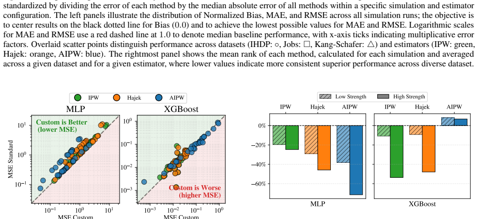
Multi-Layer Perceptron (MLP).For the experiments, we used a simple MLP architecture: •Architecture:Input layer (d= 58), two hidden layers of[64,32]units with ReLU activation, and a single output unit. •Activation: –Baseline:Standard Sigmoid function. –Ours:The custom Quartic Canonical probability mapping (Definition 3.8). • Backward Pass:While our custom ...
2048
-
[20]
Gradient Boosting (XGBoost).Unlike deep learning frameworks that rely on automatic differentiation through a computational graph, XGBoost utilizes a second-order approximation for tree boosting and requires the explicit analytical gradient (g) and Hessian (h) of the objective with respect to the raw logits z. Thanks to our canonical link, these derivative...
-
[21]
Training Methodology & Cross-Fitting.To avoid overfitting and ensure valid inference, we employed a K-fold cross-fitting strategy (typically K= 2 or K= 10 depending on sample size) as recommended by Chernozhukov et al. (2018). For each fold, the propensity model was trained on the remaining K−1 folds and used to predict propensity scores for the held-out ...
2018
-
[22]
For each model and benchmark configuration, we evaluated a grid of parameters (e.g., regularization strengthC, learning rate etc.)
Hyperparameter Tuning.Hyperparameters were selected via a grid search procedure. For each model and benchmark configuration, we evaluated a grid of parameters (e.g., regularization strengthC, learning rate etc.). The optimal combination was selected by minimizing therespective training objective(Log-Loss for standard models, and the specific Proper Scorin...
-
[23]
Outcome Modeling.For AIPW estimator we need to model outcome. We employed distinct outcome models tailored to the dimensionality of each benchmark: • Low-Dimensional (IHDP, Jobs, Kang & Schafer):We used standard Linear Regression to estimate potential outcomes µ0(x)andµ 1(x). • High-Dimensional (ACIC 2017):We utilized Lasso Regression (L1-regularized line...
2017
-
[24]
stress test
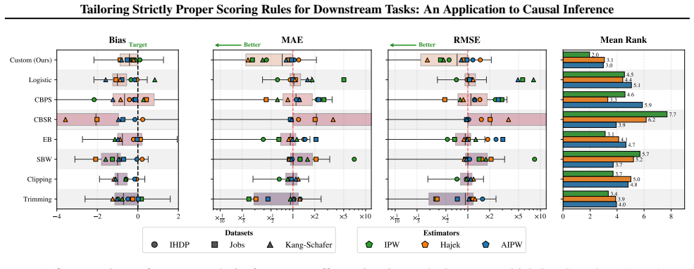
Estimators with Direct Weights (SBW, EB).For methods that learn balancing weights W directly (instead of propensity scores e), we adapted the standard estimators to utilize these learned weights Wi in place of the inverse probability terms (1/ˆei or 1/(1−ˆei)). This adaptation allows us to evaluate weight-based methods within the same doubly robust framew...
2017
-
[25]
Integral of the Weight FunctionRecall wℓ(p) = 2 p2 + 2 p3 + 2 (1−p)2 + 2 (1−p)3 . We integrate term by term, setting the constant of integration to zero to enforce symmetryσ ℓ(0) = 0.5: z= Z 2p−2 + 2p−3 + 2(1−p) −2 + 2(1−p) −3 dp =− 2 p − 1 p2 + 2 1−p + 1 (1−p) 2 = 1 (1−p) 2 − 1 p2 + 2 1 1−p − 1 p .(58)
-
[26]
Since p∈(0,1) , we have u≥4
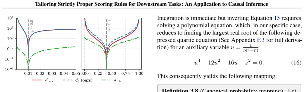
Change of Variable (The Quartic Equation)Let u= 1 p(1−p). Since p∈(0,1) , we have u≥4 . We rewrite the terms of zusingu. Note that 1 1−p − 1 p = 2p−1 p(1−p) =u(2p−1). Similarly, the squared term isu 2(2p−1). Thus: z= (u 2 + 2u)(2p−1).(59) Squaring both sides eliminates the dependence on the sign of(2p−1): z2 = (u2 + 2u)2(2p−1) 2.(60) Substituting the iden...
-
[27]
complete the square
Analytic Solution via Ferrari’s Method 33 Tailoring Strictly Proper Scoring Rules for Downstream Tasks: An Application to Causal Inference We solve the quartic equation u4 −12u 2 −16u−z 2 = 0 using Ferrari’s method. The goal is to rewrite the equation as the equality of two perfect squares. First, we move the linear and constant terms to the right side an...
-
[28]
This allows us to reduce the equation from degree 4 to degree 2
Recoveringufrom the Perfect Square The purpose of finding the root v of the resolvent cubic is to force the right-hand side of our quartic equation to become a perfect square. This allows us to reduce the equation from degree 4 to degree 2. Recall our equation from step 3: (u2 +y) 2 = (2y+ 12)u 2 + 16u+ (y 2 +z 2).(70) By setting y= 2v−2 , we ensured the ...
-
[29]
Bias-Only
Recovering the Probability We now invert the variable transformation to recover the probabilityp. Recall the definition: u= 1 p(1−p) .(77) Rearranging this equation yields a standard quadratic equation in terms ofp: p(1−p) = 1 u p2 −p+ 1 u = 0.(78) Solving forpusing the quadratic formula: p= 1± q 1− 4 u 2 .(79) 35 Tailoring Strictly Proper Scoring Rules f...
-
[30]
Integral of the Weight FunctionWe integrate the weight function to findz=σ −1 ℓ (p): z= Z 2 p2 + 2 (1−p) 2 dp =− 2 p + 2 1−p = −2(1−p) + 2p p(1−p) = 2(2p−1) p(1−p) .(87)
-
[31]
Rearranging the terms: zp(1−p) = 4p−2 zp−zp 2 = 4p−2 zp2 + (4−z)p−2 = 0.(88) This is a standard quadratic equation Ap2 +Bp+C= 0 with A=z , B= 4−z , and C=−2
Inversion (The Quadratic Equation)To find the inverse link p=σ −1 ℓ (z), we solve Equation (87) for p. Rearranging the terms: zp(1−p) = 4p−2 zp−zp 2 = 4p−2 zp2 + (4−z)p−2 = 0.(88) This is a standard quadratic equation Ap2 +Bp+C= 0 with A=z , B= 4−z , and C=−2 . Calculating the discriminant ∆: ∆ = (4−z) 2 −4(z)(−2) = 16−8z+z 2 + 8z=z 2 + 16.(89) Since∆ =z ...
discussion (0)
Sign in with ORCID, Apple, or X to comment. Anyone can read and Pith papers without signing in.