REVIEW 4 major objections 6 minor 49 references
The paper proposes that under a misspecified governing PDE, the true solution operator can be decomposed into a physics-based prior operator and a learnable correction operator, and that training a serial DeepONet with the correction placed
Reviewed by Pith at T0; open to challenge. T0 means a machine referee read the full paper against a public rubric. the ladder, T0–T4 →
A serial DeepONet framework decomposes a solution operator into a physics-based prior plus a learned correction, reporting reduced errors under misspecified PDEs.
T0 review reviewed 2026-08-04 challenge →
load-bearing objection A promising operator-correction idea undermined by a central mismatch between the claimed solution-space decomposition and the actual losses. the 4 major comments →
Physics-guided correction for operator learning under model misspecification
The pith
A machine-rendered reading of the paper's core claim, the machinery that carries it, and where it could break.
The reading
Core claim
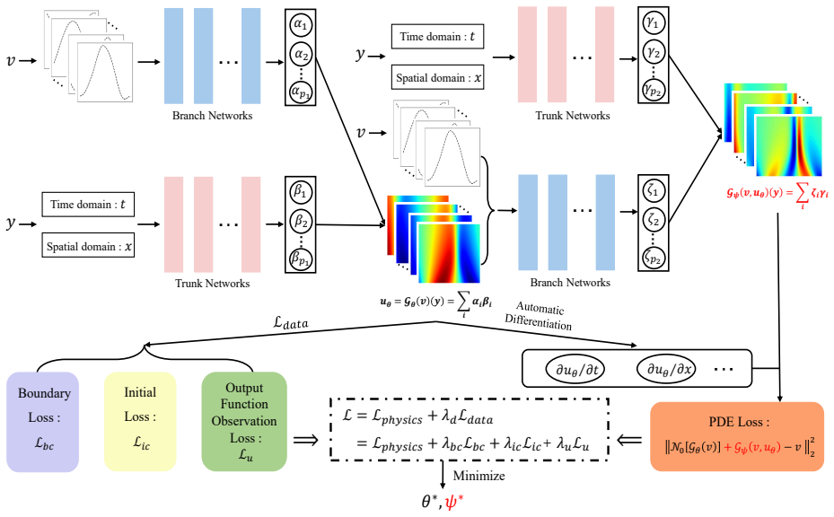
The central claim is that model misspecification in operator learning can be corrected not by changing the PDE but by learning an additive operator on top of a physics-induced prior. Specifically, the paper sets N† ≈ Gθ + Gψ, where Gθ approximates the inverse of a possibly wrong differential operator N0 and Gψ(v, Gθ(v)) approximates the discrepancy N† − N†0. Training minimizes L_physics = ||N0[Gθ(v)] + Gψ(v, uθ) − v||² plus a data loss L_data = ||Gθ(v)(y_obs) − u(y_obs)||². The paper reports that when the prior PDE is misspecified (wrong reaction term, omitted advection or diffusion, Newtonian instead of power-law viscosity, or linear instead of hyperelastic constitutive law), the corrected
What carries the argument
The load-bearing construction is a serial DeepONet: a trunk-branch network Gθ maps the input function v (sampled at sensors) to a prior predicted solution uθ; a second trunk-branch network Gψ takes both v and uθ (sampled on a coarse grid) and produces an additive correction. The correction is inserted into the residual of the prior differential operator N0, so the physics loss becomes N0[uθ] + Gψ(v, uθ) − v, and both networks are trained jointly with a data term on uθ. This design makes the correction state-dependent—it can learn missing nonlinear or derivative terms as functions of the current solution—while the prior operator still imposes the known part of the physics.
Load-bearing premise
The load-bearing premise is that the training loss as written drives the full corrected sum Gθ+Gψ toward the data, even though the data term in Eq. (2) is applied only to Gθ.
What would settle it
Train the exact serial DeepONet with the data loss moved from Gθ alone to Gθ+Gψ (the corrected prediction), keeping all other settings fixed; if the error does not stay at or below the reported levels, then the reported gains depend on supervision that the stated loss function does not provide.
If this is right
- If the decomposition works as intended, physics-informed operator learning no longer requires the prescribed PDE to be exactly right: approximate models become usable priors.
- The correction operator recovers interpretable missing terms (e.g., -k_r u, u ∂_x u, ν ∂_xx u), so the framework doubles as a data-driven discrepancy-discovery tool.
- Because the formulation is architecture-independent, the same prior-plus-correction idea extends to other neural operators and even classical numerical solvers as the prior.
- Sparse and noisy observations are shown to be tolerable: ensemble uncertainty widens but the mean stays close to the reference, suggesting a practical route to uncertainty quantification for imperfect models.
- In the hyperelasticity benchmark, the corrected model beats a standard data-only DeepONet under the same limited observations, indicating that combining an approximate physics prior with a learned correction extracts more from data than pure regression.
Where Pith is reading between the lines
- The stated training objective leaves the corrected sum Gθ+Gψ unsupervised: L_data only constrains Gθ, so the reported numerical gains rest on the physics residual indirectly pulling the sum toward the data. A direct test is to add the data loss to Gθ+Gψ; if accuracy is maintained or improved, the decomposition is more reliably enforced.
- The framework can be viewed as a model-discrepancy method at the operator level, conceptually parallel to classical Bayesian calibration—but it learns a functional correction without parameter sampling.
- A testable extension is to apply the same serial correction to time-dependent problems with parameter drift by letting the correction depend on a time index or latent parameter; the paper's examples are mostly steady or single-parameter, so dynamic drift remains open.
- The state-dependent conditioning (v, uθ) suggests the correction learns a closure term; one could inspect Gψ to see whether it converges to the analytic missing term as data increase, which would provide a falsifiable check on identifiability.
Editorial analysis
A structured set of objections, weighed in public.
Referee Report
Summary. The paper proposes a physics-guided operator correction framework for operator learning under model misspecification. The true solution operator is decomposed into a prior operator, induced by an approximate PDE model, and a learnable correction operator; the authors instantiate this with a serial DeepONet in which the first network produces the prior prediction u_θ and the second produces a correction conditioned on both the input function and u_θ. The training objective combines a physics residual built from the prior operator plus the correction, and a data-consistency loss. Numerical experiments on diffusion-reaction, Burgers, cavity flow, and hyperelasticity report that the corrected model substantially reduces errors relative to the misspecified baseline, and additional tests address sparse/noisy observations and deep-ensemble uncertainty.
Significance. The conceptual idea of correcting a prior solution operator rather than re-learning the full map is timely, and the serial DeepONet realization is a natural implementation. The four benchmark problems cover usefully different types of misspecification, and the sparse/noisy observation experiments address practical robustness. However, the central training objective as written does not train the corrected prediction that the paper claims to evaluate: the data loss supervises only G_θ, and the physics loss places G_ψ in residual/source space rather than solution space. Consequently, the reported numerical improvements are not derivable from the stated method. If the formulation is corrected and the experiments re-run, the framework could be a useful contribution; in its current form the central claim is not supported.
major comments (4)
- [§2.2, Eq. (2); Algorithm 1, line 5] The data-consistency loss is defined on G_θ(v)(y_obs) alone, and Algorithm 1 confirms this. The final corrected prediction G_θ(v)+G_ψ(v,u_θ) is never compared with the observed solutions u. Thus nothing in the objective enforces the stated target N†[v]≈G_θ(v)+G_ψ(v,u_θ). The numerical results cannot be attributed to the described training procedure. The data loss must be defined on the corrected prediction, or the corrected prediction must be supervised by an additional term.
- [§2.2, Eq. (1)] Eq. (1) imposes N_0[G_θ(v)] + G_ψ(v,u_θ) - v = 0. This treats G_ψ as an additive correction to the residual/source space, not as the solution-space discrepancy N†[v]-N_0†[v] defined in §2.1. If G_θ actually approximates the prior solution operator, then N_0[G_θ(v)]≈v and minimizing Eq. (1) drives G_ψ to zero. If instead G_θ is fitted to the true data as in Eq. (2), then G_ψ is forced to absorb the prior-model residual N_0[G_θ]-v, not the solution discrepancy. Either way, the training objective is inconsistent with the claimed decomposition. The authors need to derive Eq. (1) from the decomposition or replace it with a residual that acts on the corrected solution, e.g. N_0[G_θ+G_ψ]-v.
- [§3.1 and §3.2] The reported correction targets are inconsistent with the stated misspecification. In the diffusion-reaction example the prior is D∂²u - k_r = v and the true model is D∂²u - k_r u = v, so the residual discrepancy is k_r(1-u), not -k_r u; yet the paper defines ϕ=-k_r u as the correction quantity. In Burgers Case C, the prior omits diffusion, so the correction needed in Eq. (1) is -ν∂²u/∂x², while the text lists +ν∂²u/∂x². These sign/target mismatches mean the experiments do not implement the discrepancy described in §2.1, and the tables cannot be interpreted as validating the proposed correction.
- [§2.1, Fig. 1] The schematic in Fig. 1 shows the corrected prediction as G_θ(v) ⊕ G_ψ(v,u_θ), and the caption states that this combination approximates the true operator. But the training diagram in Fig. 2 places the data loss on u_θ only, and the physics loss on N_0[G_θ]+G_ψ. The two figures therefore depict different training objectives. The manuscript needs a single, consistent statement of what is optimized.
minor comments (6)
- [Abstract/Introduction] The phrase 'usually requires typically' is redundant; the sentence should be rewritten.
- [§3.1] Typo: 'manifactured solutions' should be 'manufactured solutions'.
- [§3, Table 1] The Adam hyperparameters are given as β_1=0.999 and β_2=0.999. This is unusual; standard values are β_1=0.9, β_2=0.999. Please clarify or correct.
- [§3.1, Table 2] The table header lists 'f' but the text and equations use v for the source term; please unify notation.
- [§3.3, Table 4] The pressure error is reported as '0.01±0.01%' and '0.80%±0.04%', which is inconsistent formatting; also clarify whether these are percentages or relative L2 errors.
- [General] No code or data availability statement is provided. Given the sensitivity of the experiments to the training objective, releasing code would materially help reproducibility.
Circularity Check
No significant circularity: the correction operator is learned from data and the self-citations are not load-bearing; the Eq. (1)-(2) supervision gap is a correctness issue, not a circular reduction.
full rationale
The paper's central decomposition N†[v] = N0†[v] + (N†[v] − N0†[v]) (Section 2.1) is an algebraic identity, but it is used as a modeling ansatz rather than as a derivation of the numerical results; the correction operator Gψ is fitted from data, not derived from the claimed target. The training objective in Eqs. (1)-(2) is inconsistent with the claimed decomposition: Eq. (2) supervises only Gθ(v), and Eq. (1) drives Gψ toward the source-space residual v − N0[Gθ], not toward the solution-space discrepancy N†[v] − N0†[v]. This is a potentially serious correctness gap, but it is not circularity: no equation in the paper makes the reported prediction equal to its input by construction, and no fitted parameter is relabeled as a prediction. The citations to prior work by Boullé et al. ([10, 29-32, 46]) are contextual—related-work pointers and benchmark setup—and are not used to justify the correction framework itself. Numerical benchmarks rely on external datasets and solvers, so the results are not forced by a self-citation chain. Therefore, no circular step is identified.
Axiom & Free-Parameter Ledger
free parameters (3)
- Loss weights λ_bc, λ_ic, λ_u, λ_e, λ_d =
λ_bc=1, λ_ic=λ_u=50 (Burgers); λ_e=100, λ_u=100000, λ_bc=1 (hyperelastic)
- DeepONet truncation p1=p2 and network width/depth =
p1=p2=100; depth 4; widths 64, 128, 256 per problem in Table 1
- Observation and collocation counts =
e.g., 101 sensors for diffusion-reaction, 51×51 grid for uθ in Burgers, 250 interior velocity points for cavity flow
axioms (3)
- domain assumption The inverse solution operators N† and N0† exist and are well approximated by neural operators Gθ and Gψ.
- ad hoc to paper Adding Gψ to the prior residual N0[Gθ] in Eq. (1) is equivalent to correcting the solution operator.
- ad hoc to paper The input function v can be evaluated at spatio-temporal collocation points y_f even when v is defined only in space (e.g., Burgers initial condition).
Cite this review
Pith. "Pith review of Physics-guided correction for operator learning under model misspecification." pith.science (2026). https://pith.science/paper/SYHD4KBT
@misc{pith2026260603469,
  author       = {Pith},
  title        = {Pith review of: Physics-guided correction for operator learning under model misspecification},
  year         = {2026},
  howpublished = {\url{https://pith.science/paper/SYHD4KBT}},
  note         = {Machine review of arXiv:2606.03469}
}
read the original abstract
Physics-informed operator learning provides an efficient framework for approximating solution operators of partial differential equations by combining observational data with governing physical laws. However, most existing methods implicitly assume that the prescribed governing equation is accurate. This assumption may fail in practical applications, where model simplifications, missing physical effects, parameter drift, or incomplete constitutive relations can lead to model misspecification. In this work, we propose a physics-guided operator correction framework for learning solution operators under misspecified governing equations. At the operator level, the target mapping is decomposed into a prior operator induced by an approximate physical model and a learnable correction operator that accounts for the remaining discrepancy. We realize the operator model correction using a serial DeepONet architecture, where the first DeepONet provides a solution prediction and the second DeepONet learns an additive correction conditioned on both the input function and the solution prediction. The learned correction is incorporated into the physics residual and trained together with data-consistency constraints, allowing the model to retain useful physical structure while adapting to inaccurate governing equations. Numerical experiments on diffusion-reaction, Burgers, cavity flow, and hyperelastic problems show that the proposed method substantially reduces errors induced by misspecified physics. Additional tests under sparse and noisy observations further demonstrate the robustness of the framework and its ability to provide informative uncertainty estimates through deep ensembles.
Figures



Reference graph
Works this paper leans on
-
[1]
G. K. Batchelor, An introduction to fluid dynamics, Cambridge University Press, 2000
2000
-
[2]
F. P . Incropera, D. P . DeWitt, T. L. Bergman, A. S. Lavine, et al., Fundamentals of heat and mass transfer, Wiley New York, 1996
1996
-
[3]
R. B. Bird, Transport phenomena, Appl. Mech. Rev. 55 (2002) 1–4
2002
-
[4]
J. N. Goodier, P . Hodge Jr, Elasticity and plasticity: The mathematical theory of elasticity and the mathematical theory of plasticity, Dover Publications, 2016
2016
-
[5]
D. E. Keyes, L. C. McInnes, C. Woodward, W. Gropp, E. Myra, M. Pernice, J. Bell, J. Brown, A. Clo, J. Connors, et al., Multiphysics simulations: Challenges and opportunities, Int. J. High Perform. Comput. Appl. 27 (2013) 4–83
2013
-
[6]
Raissi, P
M. Raissi, P . Perdikaris, G. E. Karniadakis, Physics-informed neural networks: A deep learning frame- work for solving forward and inverse problems involving nonlinear partial differential equations, J. Comput. Phys. 378 (2019) 686–707
2019
-
[7]
G. E. Karniadakis, I. G. Kevrekidis, L. Lu, P . Perdikaris, S. Wang, L. Yang, Physics-informed machine learning, Nat. Rev. Phys. 3 (2021) 422–440
2021
-
[8]
Kovachki, Z
N. Kovachki, Z. Li, B. Liu, K. Azizzadenesheli, K. Bhattacharya, A. Stuart, A. Anandkumar, Neural operator: Learning maps between function spaces with applications to PDEs, J. Mach. Learn. Res. 24 (2023) 1–97
2023
-
[9]
N. B. Kovachki, S. Lanthaler, A. M. Stuart, Operator learning: Algorithms and analysis, in: Handbook of Numerical Analysis, volume 25, Elsevier, 2024, pp. 419–467
2024
-
[10]
Boullé, A
N. Boullé, A. Townsend, A mathematical guide to operator learning, in: Handbook of Numerical Analysis, volume 25, Elsevier, 2024, pp. 83–125
2024
-
[11]
L. Lu, P . Jin, G. Pang, Z. Zhang, G. E. Karniadakis, Learning nonlinear operators via DeepONet based on the universal approximation theorem of operators, Nat. Mach. Int. 3 (2021) 218–229
2021
-
[12]
Z. Li, N. B. Kovachki, K. Azizzadenesheli, B. liu, K. Bhattacharya, A. Stuart, A. Anandkumar, Fourier neural operator for parametric partial differential equations, in: International Conference on Learning Representations, 2021
2021
-
[13]
Haghighat, U
E. Haghighat, U. bin Waheed, G. Karniadakis, En-deeponet: An enrichment approach for enhancing the expressivity of neural operators with applications to seismology, Comput. Methods Appl. Mech. Eng. 420 (2024) 116681
2024
-
[14]
Y. Qiu, N. Bridges, P . Chen, Derivative-enhanced deep operator network, in: Advances in Neural Information Processing Systems, volume 37, 2024, pp. 20945–20981
2024
-
[15]
A. Tran, A. Mathews, L. Xie, C. S. Ong, Factorized fourier neural operators, in: International Conference on Learning Representations, 2023
2023
-
[16]
Z. Li, N. Kovachki, K. Azizzadenesheli, B. Liu, A. Stuart, K. Bhattacharya, A. Anandkumar, Multipole graph neural operator for parametric partial differential equations, in: Advances in Neural Information Processing Systems, volume 33, 2020, pp. 6755–6766
2020
-
[17]
Vaswani, N
A. Vaswani, N. Shazeer, N. Parmar, J. Uszkoreit, L. Jones, A. N. Gomez, Ł. Kaiser, I. Polosukhin, Attention is all you need, in: Advances in Neural Information Processing Systems, volume 30, 2017. 18
2017
-
[18]
R. Bommasani, D. A. Hudson, E. Adeli, R. Altman, S. Arora, S. von Arx, M. S. Bernstein, J. Bohg, A. Bosselut, E. Brunskill, et al., On the opportunities and risks of foundation models, arXiv preprint arXiv:2108.07258 (2021)
Pith/arXiv arXiv 2021
-
[19]
B. Shih, A. Peyvan, Z. Zhang, G. E. Karniadakis, Transformers as neural operators for solutions of differential equations with finite regularity, Comput. Methods Appl. Mech. Eng. 434 (2025) 117560
2025
-
[20]
Z. Hao, Z. Wang, H. Su, C. Ying, Y. Dong, S. Liu, Z. Cheng, J. Song, J. Zhu, Gnot: A general neural operator transformer for operator learning, in: International conference on machine learning, 2023, pp. 12556–12569
2023
-
[21]
J. Sun, Y. Liu, Z. Zhang, H. Schaeffer, Towards a foundation model for partial differential equations: Multioperator learning and extrapolation, Phys. Rev. E 111 (2025) 035304
2025
-
[22]
S. Wang, H. Wang, P . Perdikaris, Learning the solution operator of parametric partial differential equations with physics-informed deeponets, Sci. Adv. 7 (2021) eabi8605
2021
-
[23]
Z. Li, H. Zheng, N. Kovachki, D. Jin, H. Chen, B. Liu, K. Azizzadenesheli, A. Anandkumar, Physics- informed neural operator for learning partial differential equations, ACM/IMS J. Data Sci. 1 (2024) 1–27
2024
-
[24]
E. C. S. Acquesta, T. Portone, R. Dandekar, C. Rackauckas, R. Bandy, G. Huerta, I. Dytzel, Model- Form Epistemic Uncertainty Quantification for Modeling with Differential Equations: Application to Epidemiology, Technical Report, Sandia National Laboratories, 2022
2022
-
[25]
Kaszás, U
B. Kaszás, U. Feudel, T. Tél, Tipping phenomena in typical dynamical systems subjected to parameter drift, Sci. Rep. 9 (2019) 8654
2019
-
[26]
M. C. Kennedy, A. O’Hagan, Bayesian calibration of computer models, J. R. Stat. Soc. Ser. B Stat. Methodol. 63 (2001) 425–464
2001
-
[27]
Y. Ling, J. Mullins, S. Mahadevan, Selection of model discrepancy priors in bayesian calibration, J. Comput. Phys. 276 (2014) 665–680
2014
-
[28]
M. R. Ebers, K. M. Steele, J. N. Kutz, Discrepancy modeling framework: Learning missing physics, modeling systematic residuals, and disambiguating between deterministic and random effects, SIAM J. Appl. Dyn. Syst. 23 (2024) 440–469
2024
-
[29]
Boullé, D
N. Boullé, D. Halikias, S. E. Otto, A. Townsend, Operator learning without the adjoint, J. Mach. Learn. Res. 25 (2024) 1–54
2024
-
[30]
Boullé, D
N. Boullé, D. Halikias, A. Townsend, Elliptic PDE learning is provably data-efficient, Proc. Natl. Acad. Sci. U. S. A. 120 (2023) e2303904120
2023
-
[31]
Boullé, S
N. Boullé, S. Kim, T. Shi, A. Townsend, Learning Green’s functions associated with time-dependent partial differential equations, J. Mach. Learn. Res. 23 (2022) 1–34
2022
-
[32]
Boullé, A
N. Boullé, A. Townsend, Learning elliptic partial differential equations with randomized linear algebra, Found. Comput. Math. 23 (2023) 709–739
2023
-
[33]
S. H. Rudy, S. L. Brunton, J. L. Proctor, J. N. Kutz, Data-driven discovery of partial differential equations, Sci. Adv. 3 (2017) e1602614
2017
-
[34]
Champion, B
K. Champion, B. Lusch, J. N. Kutz, S. L. Brunton, Data-driven discovery of coordinates and governing equations, Proc. Natl. Acad. Sci. U. S. A. 116 (2019) 22445–22451
2019
-
[35]
L. Podina, B. Eastman, M. Kohandel, A PINN approach to symbolic differential operator discovery with sparse data, arXiv preprint arXiv:2212.04630 (2022)
Pith/arXiv arXiv 2022
-
[36]
Z. Zou, X. Meng, G. E. Karniadakis, Correcting model misspecification in physics-informed neural networks (PINNs), J. Comput. Phys. 505 (2024) 112918. 19
2024
-
[37]
D. P . Kingma, Adam: A method for stochastic optimization, arXiv preprint arXiv:1412.6980 (2014)
Pith/arXiv arXiv 2014
-
[38]
X. Meng, L. Yang, Z. Mao, J. del Águila Ferrandis, G. E. Karniadakis, Learning functional priors and posteriors from data and physics, J. Comput. Phys. 457 (2022) 111073
2022
-
[39]
J. M. Burgers, The nonlinear diffusion equation: asymptotic solutions and statistical problems, Springer Science & Business Media, 2013
2013
-
[40]
G. B. Whitham, Linear and nonlinear waves, John Wiley & Sons, 2011
2011
-
[41]
R. J. LeVeque, Finite volume methods for hyperbolic problems, Cambridge University Press, 2002
2002
-
[42]
J. Bec, K. Khanin, Burgers turbulence, Phys. Rep. 447 (2007) 1–66
2007
-
[43]
L. Wang, J. Mi, X. Meng, Z. Guo, A localized mass-conserving lattice boltzmann approach for non- newtonian fluid flows, Commun. Comput. Phys. 17 (2015) 908–924
2015
-
[44]
R. W. Ogden, Non-linear elastic deformations, Courier Corporation, 1997
1997
-
[45]
G. A. Holzapfel, Nonlinear solid mechanics: a continuum approach for engineering, Wiley, 2000
2000
-
[46]
N. Bouziani, N. Boullé, Structure-preserving operator learning, arXiv preprint arXiv:2410.01065 (2024)
Pith/arXiv arXiv 2024
-
[47]
X. Ren, X. Lyu, Mixed form based physics-informed neural networks for performance evaluation of two-phase random materials, Eng. Appl. Artif. Intell. 127 (2024) 107250
2024
-
[48]
H. P . Langtangen, G. K. Pedersen, Scaling of differential equations, Springer, 2016
2016
-
[49]
D. W. Abueidda, S. Koric, E. Guleryuz, N. A. Sobh, Enhanced physics-informed neural networks for hyperelasticity, Int. J. Numer. Meth. Eng. 124 (2023) 1585–1601. 20
2023
This paper was first reviewed by deepseek-v4-flash on August 4, 2026.
discussion (0)
Sign in with ORCID, Apple, or X to comment. Anyone can read and Pith papers without signing in.