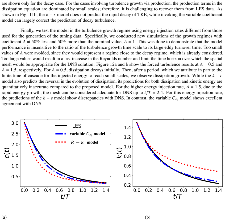
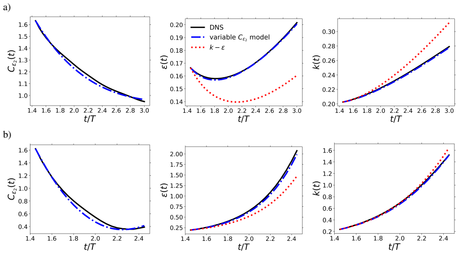
A variable-coefficient model for decay of isotropic turbulence capturing effects of finite cascade time and Reynolds number
Pith reviewed 2026-06-28 08:08 UTC · model grok-4.3
The pith
An evolution equation for C_epsilon2 captures Reynolds number and history dependence in isotropic turbulence decay due to finite cascade time.
A machine-rendered reading of the paper's core claim, the machinery that carries it, and where it could break.
Core claim
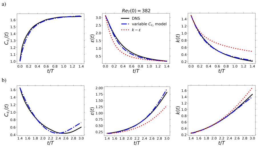
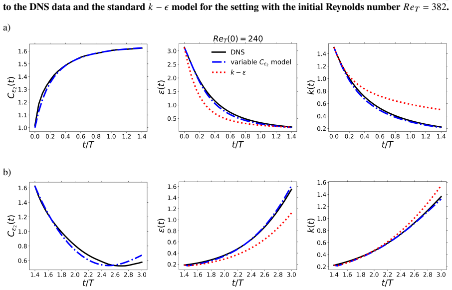
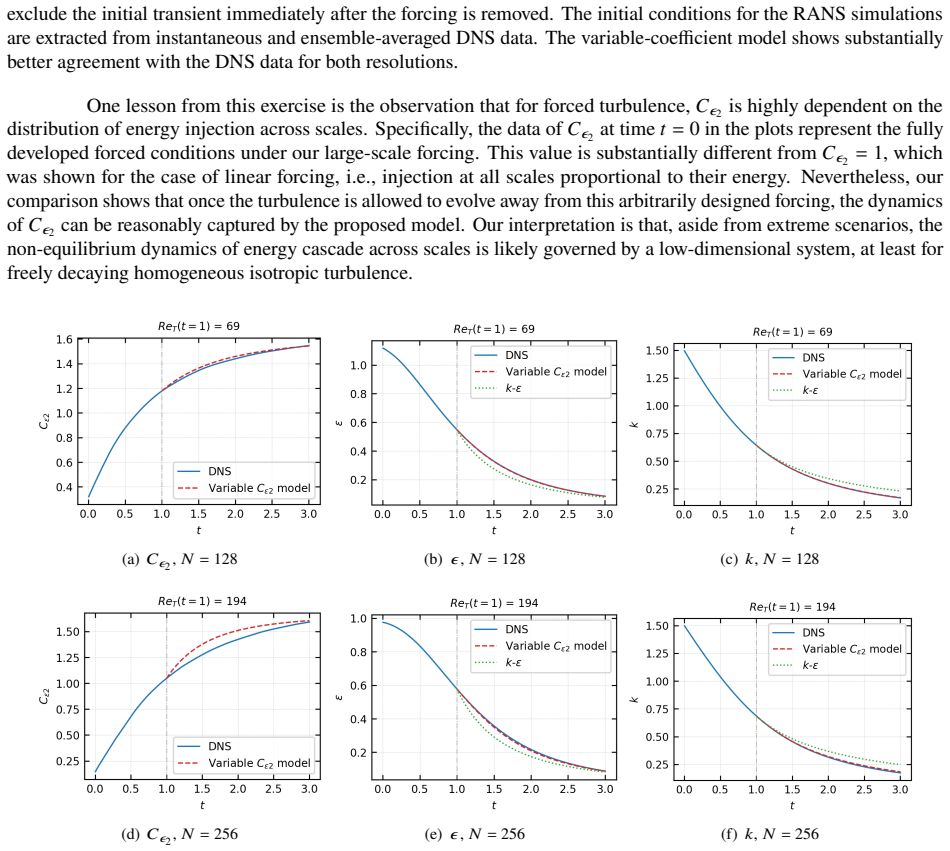
Data from high-fidelity simulations indicate that instantaneous C_epsilon2 depends on both instantaneous Reynolds number and the history of energy injection because of finite cascade time; an evolution equation for C_epsilon2 with Reynolds-dependent coefficients accurately reproduces the time evolution of dissipation and kinetic energy over wide Reynolds-number ranges and both forced and decay scenarios.
What carries the argument
Evolution equation for C_epsilon2 whose coefficients are functions of Reynolds number, constructed to encode the effects of finite cascade time and energy-injection history.
If this is right
- The variable-coefficient model reproduces dissipation and kinetic-energy decay more accurately than any fixed-value C_epsilon2 across the tested Reynolds numbers.
- The same equation works for both purely decaying turbulence and turbulence that is continuously forced.
- History dependence in C_epsilon2 is required to capture the lag between changes in large-scale energy input and the resulting change in dissipation rate.
Where Pith is reading between the lines
- The same modeling strategy could be tested in flows with sudden changes in forcing, such as grid-generated turbulence or wakes, to check whether the finite-cascade-time effect remains dominant.
- Implementation of the evolution equation inside existing k-epsilon solvers would require only a modest addition of one transport equation for C_epsilon2.
- If the Reynolds-dependent coefficients prove universal, the model might reduce the need for case-by-case tuning of decay exponents in engineering calculations.
Load-bearing premise
That the observed variations in instantaneous C_epsilon2 arise specifically from finite cascade time and the history of energy injection rather than from other unmodeled effects in the simulations.
What would settle it
A new simulation in which the time scale of the energy cascade is deliberately altered while holding Reynolds number fixed, followed by a check of whether the measured C_epsilon2 evolution still follows the proposed equation.
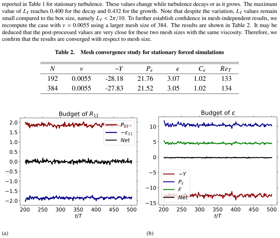
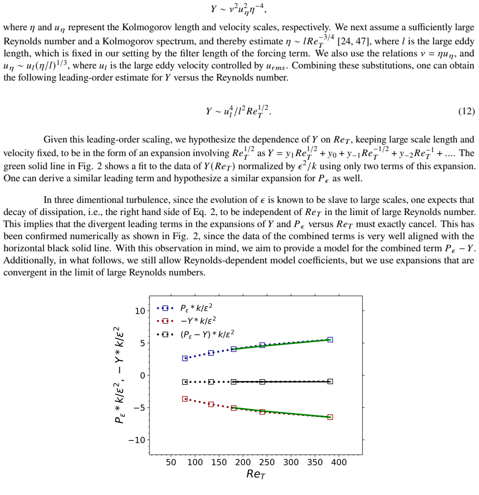
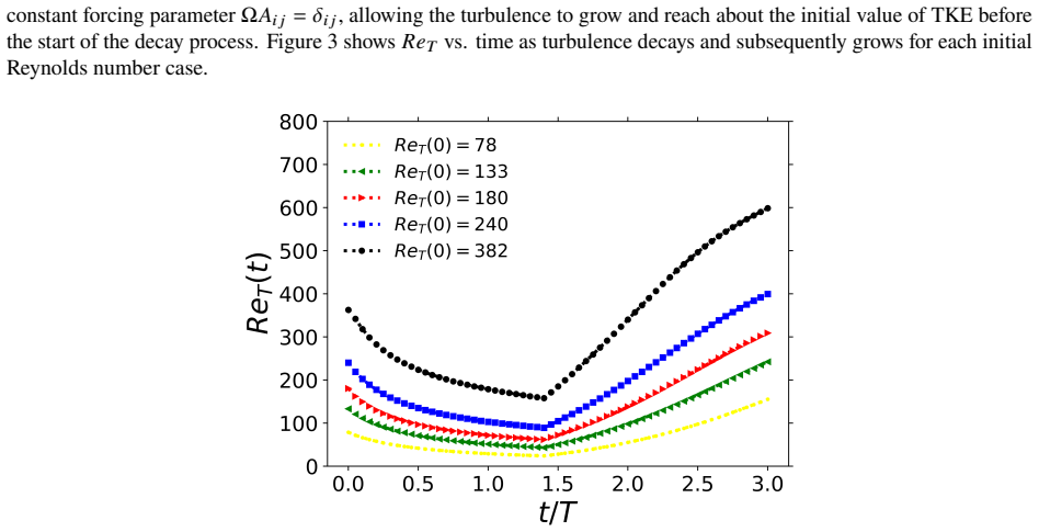
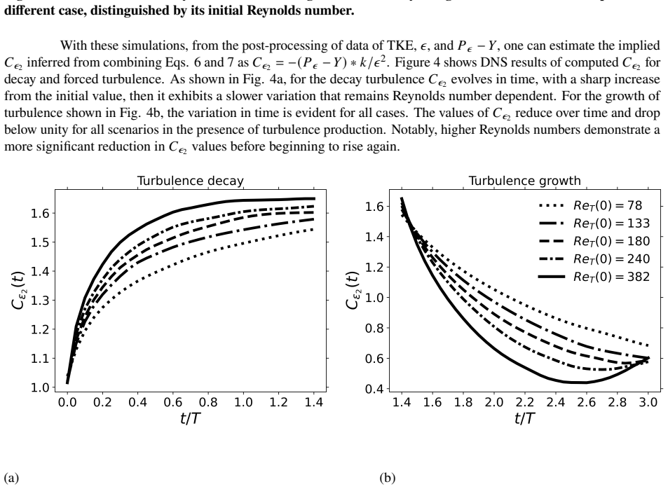
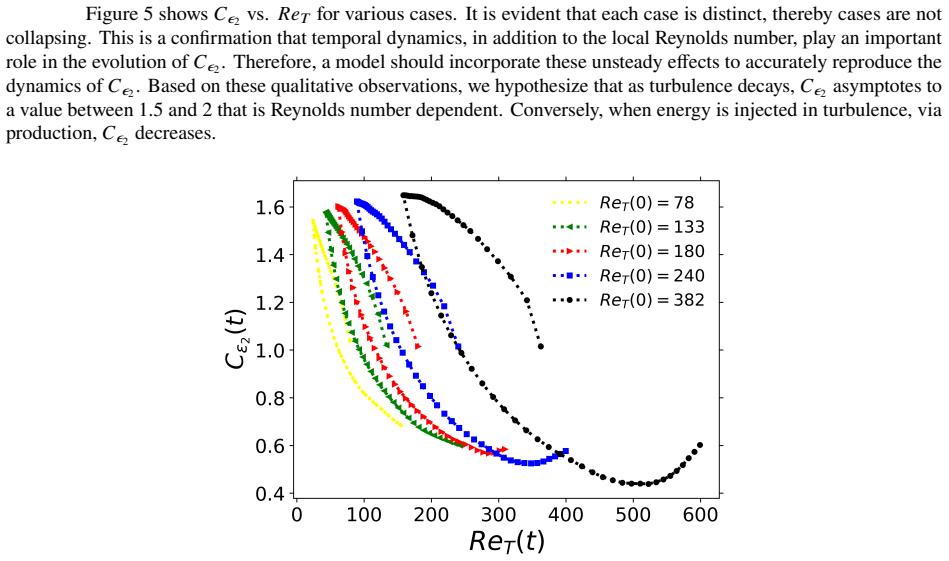
Figures
read the original abstract
We study isotropic turbulence decay in the context of the k-epsilon model, which solves the dissipation and kinetic energy equations. In modeling the dissipation equation, the coefficient C_epsilon2, suggested by Hanjalic and Launder [Journal of Fluid Mechanics, 1972] [1], is related to the temporal decay power-law by n = 1/(C_epsilon2 -1 )) and is assumed to be a constant value. In this work, we perform high-fidelity numerical simulations to examine the mathematical terms responsible for the decay of isotropic turbulence, considering both scenarios of forced and decaying turbulence. Our data suggest that the instantaneous C_epsilon2 not only depends on the instantaneous Reynolds number but is also sensitive to the history of energy injection in turbulence. We attribute these observations to the finite time required for the cascade from energetic to dissipative scales. Considering data from both decaying and growing forced turbulence, we develop an evolution equation for C_epsilon2 with Reynolds-dependent coefficients. We demonstrate that this model accurately captures the time evolution of dissipation and kinetic energy over a wide range of Reynolds numbers under a wide range of forced and decay scenarios.
Editorial analysis
A structured set of objections, weighed in public.
Referee Report
Summary. The manuscript develops a variable-coefficient extension of the k-ε model for isotropic turbulence decay. High-fidelity DNS of forced and decaying cases indicate that instantaneous C_ε2 depends on both instantaneous Reynolds number and the history of energy injection; the authors attribute this to finite cascade time and construct an evolution equation for C_ε2 whose coefficients are Reynolds-dependent. The resulting model is reported to capture the time evolution of dissipation and kinetic energy across a wide range of Reynolds numbers and forced/decay scenarios.
Significance. If the attribution to cascade time is independently confirmed and the model is shown to generalize beyond the fitting data, the work would address a known limitation of constant-coefficient k-ε closures in non-equilibrium decay, offering a more physically motivated treatment of Reynolds-number and history effects within an otherwise standard two-equation framework.
major comments (3)
- [Abstract / Model Development] Abstract, paragraph 3: the evolution equation for C_ε2 is developed from the identical DNS datasets that first revealed the Re- and history-dependence of instantaneous C_ε2. Because the coefficients are therefore fitted to those data, the subsequent claim that the model 'accurately captures' dissipation and kinetic-energy evolution on the same data does not constitute independent validation and weakens the generality asserted for 'a wide range of forced and decay scenarios'.
- [Attribution of C_ε2 dependence] Abstract, paragraph 2: the functional form of the C_ε2 evolution equation rests on the attribution that observed variations arise specifically from finite cascade time. No diagnostic (spectral transfer timescales, controlled forcing perturbations, or other isolation test) is described that separates cascade-time effects from other possible numerical or physical contributors in the DNS; without such evidence the chosen functional dependence lacks first-principles grounding.
- [Validation] Abstract, final sentence: the central claim of accurate capture is stated without any quantitative metrics (L2 errors, R² values, or reported uncertainty), error bars, or explicit cross-validation protocol. This absence makes it impossible to judge whether the reported performance supports the asserted breadth of applicability.
Simulated Author's Rebuttal
We thank the referee for the constructive comments. We address each major point below, indicating where revisions will be made to the manuscript.
read point-by-point responses
-
Referee: [Abstract / Model Development] Abstract, paragraph 3: the evolution equation for C_ε2 is developed from the identical DNS datasets that first revealed the Re- and history-dependence of instantaneous C_ε2. Because the coefficients are therefore fitted to those data, the subsequent claim that the model 'accurately captures' dissipation and kinetic-energy evolution on the same data does not constitute independent validation and weakens the generality asserted for 'a wide range of forced and decay scenarios'.
Authors: We agree that the coefficients in the evolution equation for C_ε2 were determined from the same DNS datasets used to demonstrate the model's performance. The abstract will be revised to state explicitly that the functional form and coefficients were calibrated on these forced and decaying cases, and that the reported agreement is with respect to the calibration data. We will also moderate the language on generality to reflect that broader applicability remains to be tested on independent datasets. revision: yes
-
Referee: [Attribution of C_ε2 dependence] Abstract, paragraph 2: the functional form of the C_ε2 evolution equation rests on the attribution that observed variations arise specifically from finite cascade time. No diagnostic (spectral transfer timescales, controlled forcing perturbations, or other isolation test) is described that separates cascade-time effects from other possible numerical or physical contributors in the DNS; without such evidence the chosen functional dependence lacks first-principles grounding.
Authors: The choice of functional dependence was guided by the observed sensitivity of instantaneous C_ε2 to both the current Reynolds number and the prior history of energy injection, which is consistent with a finite cascade time. No isolating diagnostics of the type mentioned were performed in this study. We will revise the abstract and discussion sections to frame the finite-cascade-time interpretation as a physically motivated hypothesis consistent with the data, while acknowledging that alternative explanations cannot be ruled out without additional targeted tests. revision: partial
-
Referee: [Validation] Abstract, final sentence: the central claim of accurate capture is stated without any quantitative metrics (L2 errors, R² values, or reported uncertainty), error bars, or explicit cross-validation protocol. This absence makes it impossible to judge whether the reported performance supports the asserted breadth of applicability.
Authors: We accept that quantitative measures of agreement are required. The revised manuscript will report L2 errors, R² values, and uncertainty estimates for the comparisons of dissipation and kinetic energy between the model and DNS across the cases. We will also describe the coefficient-fitting procedure and any cross-validation steps employed. revision: yes
Circularity Check
Evolution equation for C_epsilon2 developed from simulation data and then demonstrated on the same data
specific steps
-
fitted input called prediction
[Abstract]
"Considering data from both decaying and growing forced turbulence, we develop an evolution equation for C_epsilon2 with Reynolds-dependent coefficients. We demonstrate that this model accurately captures the time evolution of dissipation and kinetic energy over a wide range of Reynolds numbers under a wide range of forced and decay scenarios."
The evolution equation is explicitly constructed from the simulation data that revealed the Re- and history-dependence; the subsequent claim that the model 'accurately captures' the evolution therefore tests the fitted form against the same trends used to determine its coefficients, making the reported accuracy a re-expression of the input observations rather than an independent prediction.
full rationale
The paper extracts trends in instantaneous C_epsilon2 from high-fidelity simulations of forced and decaying turbulence, attributes the Re- and history-dependence to finite cascade time, constructs an evolution equation with Reynolds-dependent coefficients from those data, and then reports that the resulting model 'accurately captures' the dissipation and kinetic-energy evolution on the same class of scenarios. This matches the fitted-input-called-prediction pattern: the functional form and coefficients are calibrated to the observed trends, so the subsequent demonstration reduces to re-expressing the input data rather than an independent first-principles test. No external validation set, parameter-free derivation, or machine-checked uniqueness result is described that would break the dependence on the fitting data.
Axiom & Free-Parameter Ledger
free parameters (1)
- Reynolds-dependent coefficients in C_epsilon2 evolution equation
axioms (1)
- domain assumption Standard k-epsilon transport equations for kinetic energy and dissipation
Reference graph
Works this paper leans on
-
[1]
A Reynolds stress model of turbulence and its application to thin shear flows,
Hanjalić, K., and Launder, B. E., “A Reynolds stress model of turbulence and its application to thin shear flows,”Journal of Fluid Mechanics, Vol. 52, No. 4, 1972, p. 609–638. https://doi.org/10.1017/S002211207200268X. 21
-
[2]
Turbulence models and their applications to the prediction of internal flows: A review,
Nallasamy, M., “Turbulence models and their applications to the prediction of internal flows: A review,”Computers Fluids, Vol. 15, No. 2, 1987, pp. 151–194. https://doi.org/https://doi.org/10.1016/S0045-7930(87)80003-8
-
[3]
Bassenne,M.,Urzay,J.,Park,G.I.,andMoin,P.,“Constant-energeticsphysical-spaceforcingmethodsforimprovedconvergence to homogeneous-isotropic turbulence with application to particle-laden flows,”Physics of Fluids, Vol. 28, No. 3, 2016, p. 035114. https://doi.org/10.1063/1.4944629
-
[4]
Reynolds stress decay modeling informed by anisotropically forced homogeneous turbulence,
Homan, T., Shende, O. B., and Mani, A., “Reynolds stress decay modeling informed by anisotropically forced homogeneous turbulence,”Phys. Rev. Fluids, Vol. 9, 2024, p. 094608. https://doi.org/10.1103/PhysRevFluids.9.094608, URL https: //link.aps.org/doi/10.1103/PhysRevFluids.9.094608
-
[5]
Reynolds-stress and dissipation-rate budgets in a turbulent channel flow,
Mansour, N. N., Kim, J., and Moin, P., “Reynolds-stress and dissipation-rate budgets in a turbulent channel flow,”Journal of Fluid Mechanics, Vol. 194, 1988, p. 15–44. https://doi.org/10.1017/S0022112088002885
-
[6]
The theory of homogeneous turbulence,
Batchelor, G. K., “The theory of homogeneous turbulence,”Cambridge, 1953
1953
-
[7]
The numerical computation of turbulent flows,
Launder, B., and Spalding, D., “The numerical computation of turbulent flows,”Computer Methods in Applied Mechanics and Engineering, Vol. 3, No. 2, 1974, pp. 269–289. https://doi.org/https://doi.org/10.1016/0045-7825(74)90029-2
-
[8]
Goldberg, U., Peroomian, O., Batten, P., and Chakravarthy, S., “The k--Rt Turbulence Closure,”Engineering Applications of Computational Fluid Mechanics, Vol. 3, No. 2, 2009, pp. 175–183. https://doi.org/10.1080/19942060.2009.11015263
-
[9]
Bayesian Parameter Estimation of a k- Model for Accurate Jet-in-Crossflow Simulations,
Ray, J., Lefantzi, S., Arunajatesan, S., and Dechant, L., “Bayesian Parameter Estimation of a k- Model for Accurate Jet-in-Crossflow Simulations,”AIAA Journal, Vol. 53, 2016, pp. 1–17. https://doi.org/10.2514/1.J054758
-
[10]
On the turbulent viscosity parameter C in the k– model,
Mishra, H., and Venayagamoorthy, S. K., “On the turbulent viscosity parameter C in the k– model,”Flow, Vol. 4, 2024, p. E16. https://doi.org/10.1017/flo.2024.15
-
[11]
A comparison of standard k–𝜖 and realizable k–𝜖 turbulence models in curved and confluent channels,
Shaheed, R., Mohammadian, A., and Gildeh, H. K., “A comparison of standard k–𝜖 and realizable k–𝜖 turbulence models in curved and confluent channels,”Environmental Fluid Mechanics, Vol. 19, 2018, pp. 543–568. URL https://api.semanticscholar. org/CorpusID:125219551
2018
-
[12]
Progress in the development of a Reynolds-stress turbulence closure,
Launder, B. E., Reece, G. J., and Rodi, W., “Progress in the development of a Reynolds-stress turbulence closure,”Journal of Fluid Mechanics, Vol. 68, No. 3, 1975, p. 537–566. https://doi.org/10.1017/S0022112075001814
-
[13]
Verification and Validation of a Second-Moment-Closure Model,
Eisfeld, B., Rumsey, C., and Togiti, V., “Verification and Validation of a Second-Moment-Closure Model,”AIAA Journal, Vol. 54, No. 5, 2016, pp. 1524–1541. https://doi.org/10.2514/1.J054718
-
[14]
Differential Reynolds-Stress Modeling for Aeronautics,
Cécora, R.-D., Radespiel, R., Eisfeld, B., and Probst, A., “Differential Reynolds-Stress Modeling for Aeronautics,”AIAA Journal, Vol. 53, No. 3, 2015, pp. 739–755. https://doi.org/10.2514/1.J053250
-
[15]
Wang,J.-X.,Wu,J.-L.,andXiao,H.,“Physics-informedmachinelearningapproachforreconstructingReynoldsstressmodeling discrepanciesbasedonDNSdata,” Phys.Rev.Fluids , Vol.2, 2017, p.034603. https://doi.org/10.1103/PhysRevFluids.2.034603, URL https://link.aps.org/doi/10.1103/PhysRevFluids.2.034603
-
[16]
Formulation of the k-w Turbulence Model Revisited,
Wilcox, D. C., “Formulation of the k-w Turbulence Model Revisited,”AIAA Journal, Vol. 46, No. 11, 2008, pp. 2823–2838. https://doi.org/10.2514/1.36541
-
[17]
Hellsten, A., Laine, S., Hellsten, A., and Laine, S.,Extension of the k-omega-SST turbulence model for flows over rough surfaces, ???? https://doi.org/10.2514/6.1997-3577
-
[18]
New Advanced k-w Turbulence Model for High-Lift Aerodynamics,
Hellsten, A., “New Advanced k-w Turbulence Model for High-Lift Aerodynamics,”AIAA Journal, Vol. 43, No. 9, 2005, pp. 1857–1869. https://doi.org/10.2514/1.13754
-
[19]
Artificial neural network approach for turbulence models: A local framework,
Xie, C., Xiong, X., and Wang, J., “Artificial neural network approach for turbulence models: A local framework,”Phys. Rev. Fluids, Vol. 6, 2021, p. 084612. https://doi.org/10.1103/PhysRevFluids.6.084612, URL https://link.aps.org/doi/10.1103/ PhysRevFluids.6.084612
-
[20]
Assessmentsofk-kLTurbulenceModelBasedonMenter’sModificationtoRotta’sTwo-EquationModel,
Abdol-Hamid, K.S., “Assessmentsofk-kLTurbulenceModelBasedonMenter’sModificationtoRotta’sTwo-EquationModel,” International Journal of Aerospace Engineering, Vol. 2015, No. 1, 2015, p. 987682. https://doi.org/https://doi.org/10.1155/ 2015/987682
2015
-
[21]
Steady and Unsteady Flow Modelling Using the k-8730;kL Model,
Menter, F., Egorov, Y., and Rusch, D., “Steady and Unsteady Flow Modelling Using the k-8730;kL Model,” 2006, pp. 403–406. https://doi.org/10.1615/ICHMT.2006.TurbulHeatMassTransf.800. 22
work page doi:10.1615/ichmt.2006.turbulheatmasstransf.800 2006
-
[22]
On the Equation Governing the Rate of Turbulent Energy Dissipation,
Rodi, W., “On the Equation Governing the Rate of Turbulent Energy Dissipation,” Technical Report TM/TN/A/14, Mechanical Engineering Department, Imperial College, 1971
1971
-
[23]
The prediction of laminarization with a two-equation model of turbulence,
Jones, W., and Launder, B., “The prediction of laminarization with a two-equation model of turbulence,”International Journal of Heat and Mass Transfer, Vol. 15, No. 2, 1972, pp. 301–314. https://doi.org/https://doi.org/10.1016/0017-9310(72)90076-2
-
[24]
B.,Turbulent Flows, Cambridge University Press, 2000
Pope, S. B.,Turbulent Flows, Cambridge University Press, 2000
2000
-
[25]
The use of a contraction to improve the isotropy of grid-generated turbulence,
Comte-Bellot, G., and Corrsin, S., “The use of a contraction to improve the isotropy of grid-generated turbulence,”Journal of Fluid Mechanics, Vol. 25, No. 4, 1966, p. 657–682. https://doi.org/10.1017/S0022112066000338
-
[26]
Simple Eulerian time correlation of full-and narrow-band velocity signals in grid- generated, ‘isotropic’ turbulence,
Comte-Bellot, G., and Corrsin, S., “Simple Eulerian time correlation of full-and narrow-band velocity signals in grid- generated, ‘isotropic’ turbulence,”Journal of Fluid Mechanics, Vol. 48, No. 2, 1971, p. 273–337. https://doi.org/10.1017/ S0022112071001599
1971
-
[27]
Decayingturbulenceinanactive-grid-generatedflowandcomparisonswith large-eddy simulation,
KANG,H.S.,CHESTER,S.,andMENEVEAU,C.,“Decayingturbulenceinanactive-grid-generatedflowandcomparisonswith large-eddy simulation,”Journal of Fluid Mechanics, Vol. 480, 2003, p. 129–160. https://doi.org/10.1017/S0022112002003579
-
[28]
Freely decaying, homogeneous turbulence generated by multi-scale grids,
KROGSTAD, P.-, and DAVIDSON, P. A., “Freely decaying, homogeneous turbulence generated by multi-scale grids,”Journal of Fluid Mechanics, Vol. 680, 2011, p. 417–434. https://doi.org/10.1017/jfm.2011.169
-
[29]
DNS of rotating and non-rotating turbulent flows with synthetic inlet conditions,
Orlandi, P., “DNS of rotating and non-rotating turbulent flows with synthetic inlet conditions,”Journal of Turbulence, Vol. 14, No. 5, 2013, pp. 10–34. https://doi.org/10.1080/14685248.2013.815357
-
[30]
Lattice-Boltzmann simulation of grid-generated turbulence,
DJENIDI, L., “Lattice-Boltzmann simulation of grid-generated turbulence,”Journal of Fluid Mechanics, Vol. 552, 2006, p. 13–35. https://doi.org/10.1017/S002211200600869X
-
[31]
Direct numerical simulation of laboratory experiments in isotropic turbulence,
de Bruyn Kops, S. M., and Riley, J. J., “Direct numerical simulation of laboratory experiments in isotropic turbulence,”Physics of Fluids, Vol. 10, No. 9, 1998, pp. 2125–2127. https://doi.org/10.1063/1.869733
-
[32]
Laws of turbulence decay from direct numerical simulations,
Panickacheril John, J., Donzis, D., and Sreenivasan, K., “Laws of turbulence decay from direct numerical simulations,” , 06
-
[33]
https://doi.org/10.48550/arXiv.2106.15710
-
[34]
The decay of homogeneous isotropic turbulence,
George, W. K., “The decay of homogeneous isotropic turbulence,”Physics of Fluids A: Fluid Dynamics, Vol. 4, No. 7, 1992, pp. 1492–1509. https://doi.org/10.1063/1.858423
-
[35]
Decay of homogeneous, nearly isotropic turbulence behind active fractal grids,
Thormann, A., and Meneveau, C., “Decay of homogeneous, nearly isotropic turbulence behind active fractal grids,”Physics of Fluids, Vol. 26, No. 2, 2014, p. 025112. https://doi.org/10.1063/1.4865232
-
[36]
Multiple-Time-Scale Concepts in Turbulent Transport Modeling,
Launder, B., and Schiestel, R., “Multiple-Time-Scale Concepts in Turbulent Transport Modeling,”Turbulent Shear Flows, Vol. 2, 1980
1980
-
[37]
Klein, T., Craft, T., and Iacovides, H., “Assessment of the performance of different classes of turbulence models in a wide range of non-equilibrium flows,”International Journal of Heat and Fluid Flow, Vol. 51, 2015, pp. 229–256. https://doi.org/https: //doi.org/10.1016/j.ijheatfluidflow.2014.10.017, URL https://www.sciencedirect.com/science/article/pii/S...
-
[38]
Temperature and concentration profiles in fully turbulent boundary layers,
Kader, B., “Temperature and concentration profiles in fully turbulent boundary layers,”International Journal of Heat and Mass Transfer, Vol. 24, No. 9, 1981, pp. 1541–1544. https://doi.org/https://doi.org/10.1016/0017-9310(81)90220-9, URL https://www.sciencedirect.com/science/article/pii/0017931081902209
-
[39]
Parallel variable-density particle-laden turbulence simulation,
Pouransari, H., Mortazavi, M., and Mani, A., “Parallel variable-density particle-laden turbulence simulation,”CTR Annual Research Briefs, 2016
2016
-
[40]
General Circulation Experiments with the Primitive Equations,
Smagorinsky, J., “General Circulation Experiments with the Primitive Equations,”Monthly Weather Review, Vol. 91, No. 3, 1963, p. 99. https://doi.org/10.1175/1520-0493(1963)091<0099:GCEWTP>2.3.CO;2
-
[41]
On the application of the eddy viscosity concept in the Inertial sub-range of turbulence,
Lilly, K. E., “On the application of the eddy viscosity concept in the Inertial sub-range of turbulence,” 1966. URL https://api.semanticscholar.org/CorpusID:55104948
1966
-
[42]
Rosales,C.,andMeneveau,C.,“Linearforcinginnumericalsimulationsofisotropicturbulence: Physicalspaceimplementations and convergence properties,”Physics of Fluids, Vol. 17, No. 9, 2005, p. 095106. https://doi.org/10.1063/1.2047568
-
[43]
Linearly Forced Isotropic Turbulence,
Lundgren, T., “Linearly Forced Isotropic Turbulence,”Annual Research Briefs, 2003. 23
2003
-
[44]
A model for drift velocity mediated scalar eddy diffusivity in homogeneous turbulent flows,
Shende, O. B., Storan, L., and Mani, A., “A model for drift velocity mediated scalar eddy diffusivity in homogeneous turbulent flows,”Journal of Fluid Mechanics, Vol. 989, 2024, p. A14. https://doi.org/10.1017/jfm.2024.457
-
[45]
Uhlmann, M., and Chouippe, A., “Clustering and preferential concentration of finite-size particles in forced homogeneous- isotropic turbulence,”Journal of Fluid Mechanics, Vol. 812, 2017, p. 991–1023. https://doi.org/10.1017/jfm.2016.826
-
[46]
Harmonic analysis filtering techniques for forced and decaying homogeneous isotropic turbulence,
Kareem, W. A., Nabil, T., Izawa, S., and Fukunishi, Y., “Harmonic analysis filtering techniques for forced and decaying homogeneous isotropic turbulence,”Computers Mathematics with Applications, Vol. 65, No. 7, 2013, pp. 1059–1085. https://doi.org/https://doi.org/10.1016/j.camwa.2013.01.042
-
[47]
Entrainment in a shear-free turbulent mixing layer,
Briggs, D. A., Ferziger, J. H., Koseff, J. R., and Monismith, S. G., “Entrainment in a shear-free turbulent mixing layer,”Journal of Fluid Mechanics, Vol. 310, 1996, p. 215–241. https://doi.org/10.1017/S0022112096001784
-
[48]
Kolmogorov, A. N., “A refinement of previous hypotheses concerning the local structure of turbulence in a viscous incompressible fluid at high Reynolds number,”Journal of Fluid Mechanics, Vol. 13, No. 1, 1962, p. 82–85. https: //doi.org/10.1017/S0022112062000518
-
[49]
Donzis, D. A., Yeung, P. K., and Sreenivasan, K. R., “Dissipation and enstrophy in isotropic turbulence: Resolution effects and scaling in direct numerical simulations,”Physics of Fluids, Vol. 20, No. 4, 2008, p. 045108. https://doi.org/10.1063/1.2907227
-
[50]
Final Stage Decay of Grid-Produced Turbulence,
Tan, H. S., and Ling, S. C., “Final Stage Decay of Grid-Produced Turbulence,”The Physics of Fluids, Vol. 6, No. 12, 1963, pp. 1693–1699. https://doi.org/10.1063/1.1711011
-
[51]
Decay of isotropic turbulence in the initial period,
Batchelor, G. K., Townsend, A. A., and Taylor, G. I., “Decay of isotropic turbulence in the initial period,”Proceedings of the Royal Society of London. Series A. Mathematical and Physical Sciences, Vol. 193, No. 1035, 1948, pp. 539–558. https://doi.org/10.1098/rspa.1948.0061
-
[52]
The large-scale structure of homogeneous turbulence,
Saffman, P. G., “The large-scale structure of homogeneous turbulence,”Journal of Fluid Mechanics, Vol. 27, No. 3, 1967, p. 581–593. https://doi.org/10.1017/S0022112067000552
-
[53]
The Large-Scale Structure of Homogeneous Turbulence,
Batchelor, G. K., and Proudman, I., “The Large-Scale Structure of Homogeneous Turbulence,”Philosophical Transactions of the Royal Society of London Series A, Vol. 248, No. 949, 1956, pp. 369–405. https://doi.org/10.1098/rsta.1956.0002
-
[54]
Understanding evolution of vortex rings in viscous fluids,
Tinaikar, A., Advaith, S., and Basu, S., “Understanding evolution of vortex rings in viscous fluids,”Journal of Fluid Mechanics, Vol. 836, 2018, p. 873–909. https://doi.org/10.1017/jfm.2017.815
-
[55]
The Velocity of Viscous Vortex Rings,
Saffman, P. G., “The Velocity of Viscous Vortex Rings,”Studies in Applied Mathematics, Vol. 49, No. 4, 1970, pp. 371–380. https://doi.org/https://doi.org/10.1002/sapm1970494371
-
[56]
Power-law exponent in the transition period of decay in grid turbulence,
Djenidi, L., Kamruzzaman, M., and Antonia, R. A., “Power-law exponent in the transition period of decay in grid turbulence,” Journal of Fluid Mechanics, Vol. 779, 2015, p. 544–555. https://doi.org/10.1017/jfm.2015.428
-
[57]
On the decay of homogeneous isotropic turbulence,
Skrbek, L., and Stalp, S. R., “On the decay of homogeneous isotropic turbulence,”Physics of Fluids, Vol. 12, No. 8, 2000, pp. 1997–2019. https://doi.org/10.1063/1.870447
-
[58]
Oscillating grids as a source of nearly isotropic turbulence,
De Silva, I. P. D., and Fernando, H. J. S., “Oscillating grids as a source of nearly isotropic turbulence,”Physics of Fluids, Vol. 6, No. 7, 1994, pp. 2455–2464. https://doi.org/10.1063/1.868193
-
[59]
The decay of turbulence in a bounded domain,
Touil, H., Bertoglio, J.-P., and Shao, L., “The decay of turbulence in a bounded domain,”Journal of Turbulence, Vol. 3, 2002, N49. https://doi.org/10.1088/1468-5248/3/1/049
-
[60]
On Degeneration (Decay) of Isotropic Turbulence in an Incompressible Viscous Liquid,
Kolmogorov, A., “On Degeneration (Decay) of Isotropic Turbulence in an Incompressible Viscous Liquid,”Doklady Akademii Nauk SSSR, Vol. 31, 1941, pp. 538–541
1941
-
[61]
The role of big eddies in homogeneous turbulence,
Batchelor, G. K., “The role of big eddies in homogeneous turbulence,”Proceedings of the Royal Society of London. Series A. Mathematical and Physical Sciences, Vol. 195, No. 1043, 1949, pp. 513–532
1949
-
[62]
On non-self-similar regimes in homogeneous isotropic turbulence decay,
Meldi, M., and Sagaut, P., “On non-self-similar regimes in homogeneous isotropic turbulence decay,”Journal of Fluid Mechanics, Vol. 711, 2012, pp. 364–393
2012
-
[63]
Is grid turbulence Saffman turbulence?
KROGSTAD, P.-, and DAVIDSON, P. A., “Is grid turbulence Saffman turbulence?”Journal of Fluid Mechanics, Vol. 642, 2010, p. 373–394. https://doi.org/10.1017/S0022112009991807
-
[64]
Note on decay of homogeneous turbulence,
Saffman, P., “Note on decay of homogeneous turbulence,”Physics of fluids, Vol. 10, No. 6, 1967, pp. 1349–1349
1967
-
[65]
Davidson, P.,Turbulence: an introduction for scientists and engineers, Oxford university press, 2015. 24
2015
discussion (0)
Sign in with ORCID, Apple, or X to comment. Anyone can read and Pith papers without signing in.