Beyond False Stability: High-Noise Drift Gating for Test-Time Adversarial Defenses in Vision-Language Models
Pith reviewed 2026-06-28 11:01 UTC · model grok-4.3
The pith
High-noise feature drift in CLIP representations serves as a gating signal to selectively trigger test-time adversarial defenses, improving the clean-robust accuracy trade-off.
A machine-rendered reading of the paper's core claim, the machinery that carries it, and where it could break.
Core claim
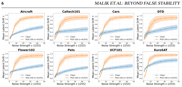
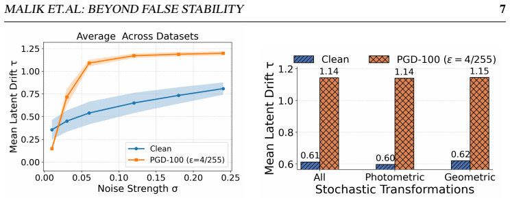
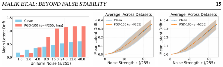
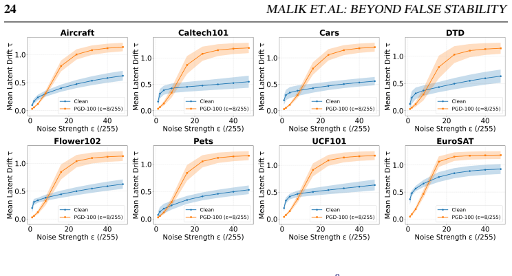
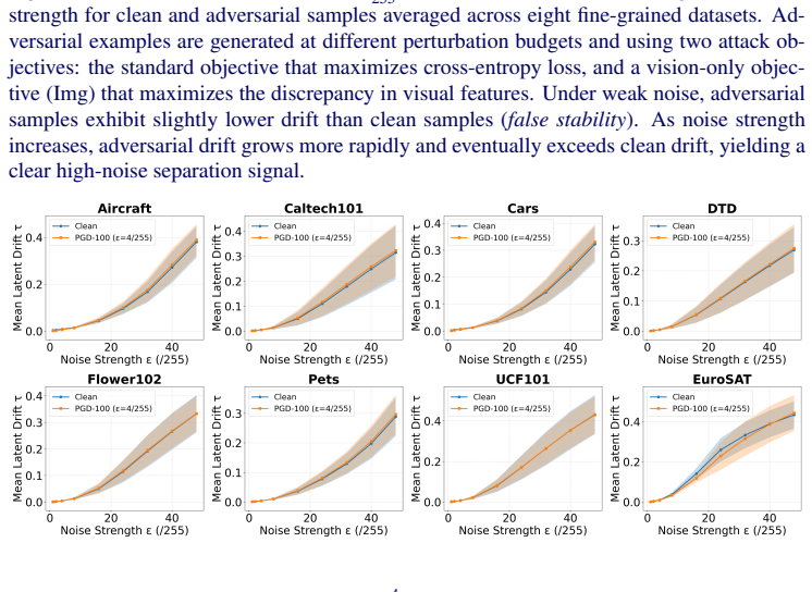
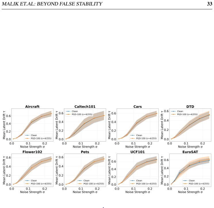
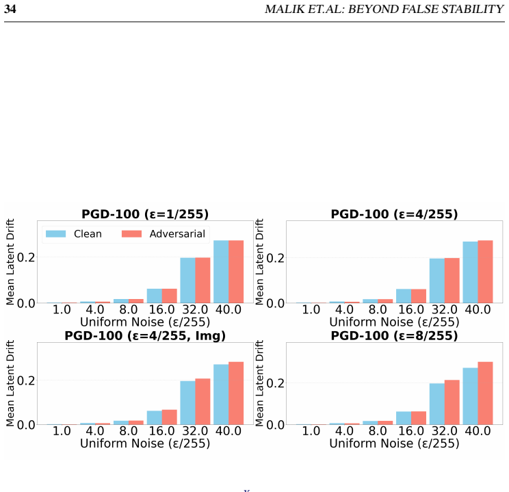
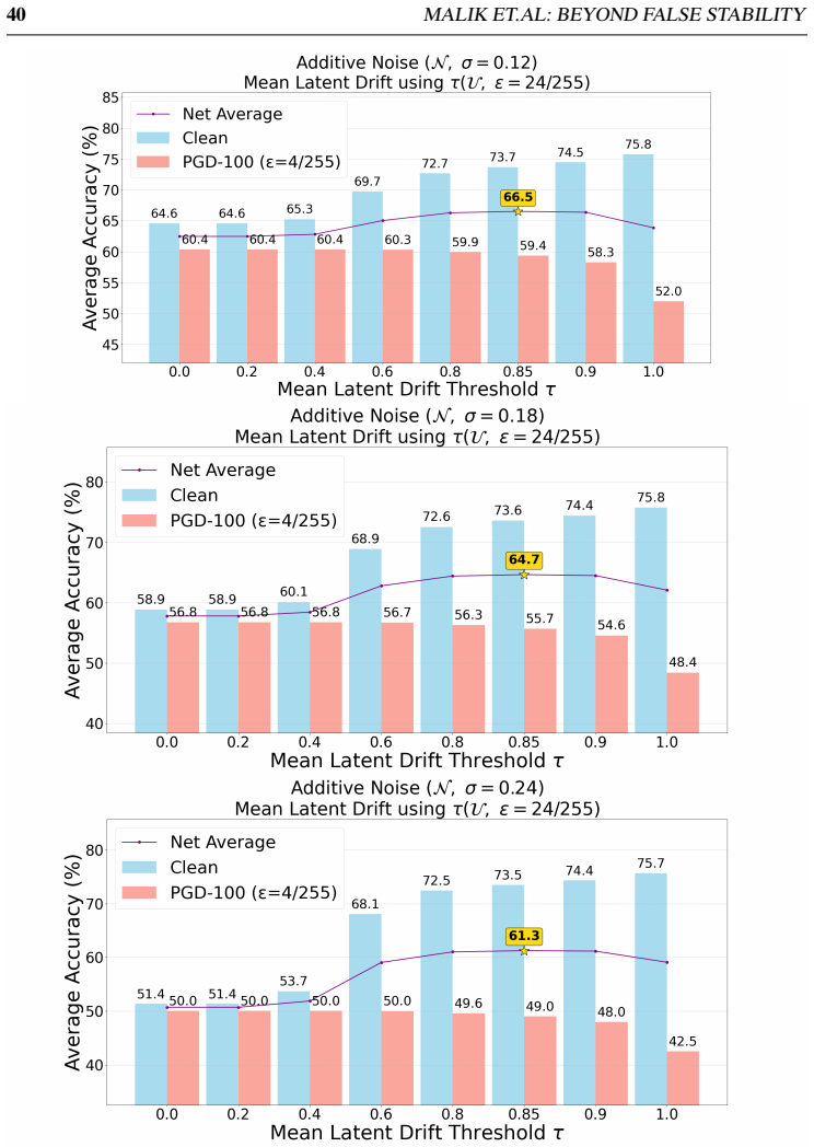
In non-robust CLIP, adversarial representations exhibit markedly higher instability under high-noise perturbations than clean representations, in contrast to the false stability observed at weak noise; this geometry-dependent transition supplies a lightweight, training-free gating signal that selectively activates test-time defenses only when high-noise drift indicates adversarial-like behavior, producing consistent gains in the clean-robust trade-off across thirteen datasets and multiple attack families.
What carries the argument
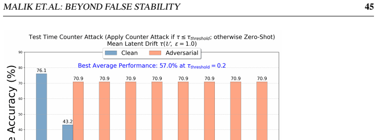
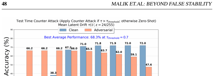
Drift-gated mechanism: a lightweight check on high-noise feature drift that gates the application of existing test-time defenses when instability exceeds clean levels.
If this is right
- The mechanism raises mean clean-plus-adversarial accuracy from 65.7 percent to 71.4 percent for counterattack defenses and from 68.4 percent to 73.2 percent for noise-anchoring on eight fine-grained datasets.
- On ImageNet and four distribution shifts the same gating lifts accuracy from 56.1 percent to 66.2 percent and from 62.1 percent to 67.6 percent.
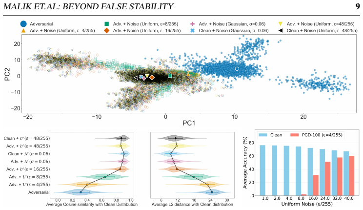
- The separation signal disappears in adversarially trained models, indicating dependence on the fragile local-basin geometry of non-robust representations.
- The transition is reproducible with both uniform and Gaussian noise as well as photometric and geometric transforms.
Where Pith is reading between the lines
- The same high-noise instability signal could be tested as a lightweight detector for other representation vulnerabilities beyond adversarial examples.
- Selective gating may lower the average compute cost of always-on test-time defenses by skipping them on clean inputs.
- If the geometry link holds, adversarially trained models may require different test-time strategies that do not rely on drift separation.
Load-bearing premise
The stability reversal from false stability at low noise to clear adversarial instability at high noise remains consistent across noise distributions, image transforms, datasets, and attack methods in non-robust CLIP models.
What would settle it
An experiment on a held-out VLM or dataset in which high-noise drift fails to separate clean from adversarial examples more reliably than low-noise drift, or in which the gating step produces no net gain in clean-plus-adversarial accuracy.
Figures


read the original abstract
Vision-language models (VLMs) such as CLIP show strong zero-shot generalization but remain highly vulnerable to adversarial attacks. Adversarial training improves robustness but is computationally expensive, motivating test-time defenses. Recent approaches exploit how CLIP's visual representations respond to stochastic perturbations: aggregating predictions across noisy views, constructing Gaussian noise-averaged anchors and interpolating features toward them, or applying counter-perturbations. These strategies improve robustness but often degrade clean accuracy, yielding an unfavorable clean-robust trade-off. We revisit stochastic test-time defenses and identify an underexplored noise-regime transition in CLIP's representation space. Prior work explored perturbations mainly in the weak-noise regime, where adversarial examples can appear unusually stable (false stability). Our analysis shows this reverses as perturbation strength grows: beyond the weak-noise regime, adversarial representations become markedly more unstable than clean ones, giving a clearer separation signal. The transition is consistent across uniform and Gaussian noise, photometric and geometric transforms, datasets, and diverse attacks. It largely disappears in adversarially trained models, suggesting it is tied to the fragile local-basin geometry of adversarial representations in non-robust CLIP. We propose a training-free, plug-in drift-gated mechanism that uses high-noise feature drift as a lightweight gating signal to trigger existing test-time defenses only when adversarial-like instability is detected. Across 13 datasets it consistently improves the clean-robust trade-off. On eight fine-grained datasets, mean clean+adversarial accuracy rises from 65.7% to 71.4% for counterattack defenses and 68.4% to 73.2% for noise-anchoring; on ImageNet and four shifted variants, from 56.1% to 66.2% and 62.1% to 67.6%.
Editorial analysis
A structured set of objections, weighed in public.
Referee Report
Summary. The paper claims that CLIP-style VLMs exhibit a noise-regime transition in which adversarial representations become markedly more unstable than clean ones beyond the weak-noise regime (consistent across noise types, transforms, datasets, and attacks), and that this transition largely vanishes under adversarial training. It introduces a training-free drift-gated mechanism that uses high-noise feature drift as a gating signal to selectively trigger existing test-time defenses (counterattack and noise-anchoring), reporting mean clean+adversarial accuracy gains from 65.7% to 71.4% and 68.4% to 73.2% on eight fine-grained datasets and from 56.1% to 66.2% / 62.1% to 67.6% on ImageNet and shifts.
Significance. If the transition is reproducible with a precisely defined instability metric and the gating improves the trade-off without implicit ensembling or post-hoc regime selection, the work supplies a lightweight, plug-in enhancement to stochastic test-time defenses that exploits the local-basin geometry of non-robust CLIP representations. The cross-condition consistency and disappearance under adversarial training would be a useful empirical observation for the field.
major comments (3)
- [Abstract; §3 (methods)] The abstract and methods description assert a 'sharp, reproducible increase' in instability and a 'consistent' transition across noise types, transforms, datasets, and attacks, yet supply neither the exact instability metric (e.g., cosine distance after N high-noise views, variance of normalized features) nor the numerical noise-strength boundary separating regimes. This is load-bearing for the central claim and for verifying that the reported accuracy lifts are attributable to the gating signal rather than extra forward passes.
- [§4 (experiments); Table 1] Table 1 / §4 results report aggregate mean clean+adversarial accuracy improvements (65.7% → 71.4%, 68.4% → 73.2%) but do not include per-dataset clean vs. adversarial breakdowns, standard deviations, or an ablation isolating the gating decision from the base defense. Without these, it is impossible to confirm that the mechanism triggers only on adversarial-like instability or that the gains are not artifacts of implicit ensembling.
- [§3.3; §4.3] The claim that the stability transition 'largely disappears in adversarially trained models' is used to attribute the phenomenon to fragile local-basin geometry, but no quantitative comparison (drift curves or tables) of AT vs. non-AT models is referenced. This evidence is required to support the geometric interpretation that underpins the gating design.
minor comments (2)
- [§3.2] Notation for the drift signal (e.g., which layer(s), normalization, exact aggregation) should be formalized with an equation in §3.2 to aid reproducibility.
- [Abstract] The abstract would be clearer if it stated the precise instability measure and the number of high-noise views used for gating.
Simulated Author's Rebuttal
Thank you for the referee's insightful comments. We address each major point below and commit to revisions that enhance clarity and completeness of the manuscript.
read point-by-point responses
-
Referee: [Abstract; §3 (methods)] The abstract and methods description assert a 'sharp, reproducible increase' in instability and a 'consistent' transition across noise types, transforms, datasets, and attacks, yet supply neither the exact instability metric (e.g., cosine distance after N high-noise views, variance of normalized features) nor the numerical noise-strength boundary separating regimes. This is load-bearing for the central claim and for verifying that the reported accuracy lifts are attributable to the gating signal rather than extra forward passes.
Authors: We thank the referee for highlighting this. The instability metric is the average cosine distance between the clean feature and features from K high-noise perturbed views (K=10 in our experiments). The regime transition is observed starting at noise strength corresponding to epsilon=0.25 for L-infty attacks or sigma=0.4 for Gaussian. We will explicitly define the metric with the formula in §3 and report the boundary values used for gating in the revised manuscript to ensure reproducibility. revision: yes
-
Referee: [§4 (experiments); Table 1] Table 1 / §4 results report aggregate mean clean+adversarial accuracy improvements (65.7% → 71.4%, 68.4% → 73.2%) but do not include per-dataset clean vs. adversarial breakdowns, standard deviations, or an ablation isolating the gating decision from the base defense. Without these, it is impossible to confirm that the mechanism triggers only on adversarial-like instability or that the gains are not artifacts of implicit ensembling.
Authors: We agree these details are important. In the revision, we will expand Table 1 to include per-dataset results with clean and adversarial accuracies separately, report standard deviations across 3 random seeds, and add an ablation study comparing the drift-gated approach to the base defense, always-trigger, and random-trigger baselines to demonstrate that gains stem from selective gating rather than ensembling. revision: yes
-
Referee: [§3.3; §4.3] The claim that the stability transition 'largely disappears in adversarially trained models' is used to attribute the phenomenon to fragile local-basin geometry, but no quantitative comparison (drift curves or tables) of AT vs. non-AT models is referenced. This evidence is required to support the geometric interpretation that underpins the gating design.
Authors: The manuscript references experiments showing the transition vanishes under AT, but we concur that explicit quantitative evidence is needed. We will include a new figure in the revision depicting drift vs. noise strength curves for both standard CLIP and adversarially trained variants, along with a table summarizing the difference in instability at high-noise regimes. revision: yes
Circularity Check
No circularity: empirical observation of drift transition with direct-measurement gating
full rationale
The paper's core contribution is an empirical identification of a high-noise instability transition in CLIP representations, followed by a training-free gating rule that triggers existing defenses when measured feature drift exceeds an (unspecified) threshold. The abstract and description contain no equations, fitted parameters, or self-citations whose load-bearing premise reduces the reported accuracy gains (65.7 % → 71.4 %, etc.) to a quantity defined by the method itself. The gating signal is constructed from observable cosine or Euclidean drift between clean and high-noise views, which is independent of the downstream defense performance it modulates. No self-definitional, fitted-input, or uniqueness-imported steps appear.
Axiom & Free-Parameter Ledger
axioms (1)
- domain assumption The observed stability transition is tied to the fragile local-basin geometry of adversarial representations in non-robust CLIP.
Reference graph
Works this paper leans on
-
[1]
Align your prompts: Test-time prompting with distribution alignment for zero-shot generalization.Advances in Neural Information Processing Systems, 36:80396–80413, 2023
Jameel Abdul Samadh, Mohammad Hanan Gani, Noor Hussein, Muhammad Uzair Khattak, Muhammad Muzammal Naseer, Fahad Shahbaz Khan, and Salman H Khan. Align your prompts: Test-time prompting with distribution alignment for zero-shot generalization.Advances in Neural Information Processing Systems, 36:80396–80413, 2023
2023
-
[2]
Obfuscated gradients give a false sense of security: Circumventing defenses to adversarial examples
Anish Athalye, Nicholas Carlini, and David Wagner. Obfuscated gradients give a false sense of security: Circumventing defenses to adversarial examples. InInternational conference on machine learning, pages 274–283. PMLR, 2018
2018
-
[3]
Semantic- enhanced image clustering
Shaotian Cai, Liping Qiu, Xiaojun Chen, Qin Zhang, and Longteng Chen. Semantic- enhanced image clustering. InProceedings of the AAAI conference on artificial intelli- gence, volume 37, pages 6869–6878, 2023
2023
-
[4]
Towards evaluating the robustness of neural net- works
Nicholas Carlini and David Wagner. Towards evaluating the robustness of neural net- works. In2017 ieee symposium on security and privacy (sp), pages 39–57. Ieee, 2017. 16MALIK ET.AL: BEYOND FALSE STABILITY
2017
-
[5]
Describing textures in the wild
Mircea Cimpoi, Subhransu Maji, Iasonas Kokkinos, Sammy Mohamed, and Andrea Vedaldi. Describing textures in the wild. InProceedings of the IEEE Conference on Computer Vision and Pattern Recognition, pages 3606–3613, 2014
2014
-
[6]
Certified adversarial robustness via randomized smoothing
Jeremy Cohen, Elan Rosenfeld, and Zico Kolter. Certified adversarial robustness via randomized smoothing. Ininternational conference on machine learning, pages 1310–
-
[7]
Reliable evaluation of adversarial robustness with an ensemble of diverse parameter-free attacks
Francesco Croce and Matthias Hein. Reliable evaluation of adversarial robustness with an ensemble of diverse parameter-free attacks. InInternational conference on machine learning, pages 2206–2216. PMLR, 2020
2020
-
[8]
Imagenet: A large-scale hierarchical image database
Jia Deng, Wei Dong, Richard Socher, Li-Jia Li, Kai Li, and Li Fei-Fei. Imagenet: A large-scale hierarchical image database. In2009 IEEE Conference on Computer Vision and Pattern Recognition, pages 248–255. IEEE, 2009
2009
-
[9]
Boosting adversarial attacks with momentum
Yinpeng Dong, Fangzhou Liao, Tianyu Pang, Hang Su, Jun Zhu, Xiaolin Hu, and Jian- guo Li. Boosting adversarial attacks with momentum. InProceedings of the IEEE conference on computer vision and pattern recognition, pages 9185–9193, 2018
2018
-
[10]
Adversarial robustness as a prior for learned representations
Logan Engstrom, Andrew Ilyas, Shibani Santurkar, Dimitris Tsipras, Brandon Tran, and Aleksander Madry. Adversarial robustness as a prior for learned representations. arXiv preprint arXiv:1906.00945, 2019
-
[11]
Learning generative visual models from few training examples: An incremental bayesian approach tested on 101 object categories
Li Fei-Fei, Rob Fergus, and Pietro Perona. Learning generative visual models from few training examples: An incremental bayesian approach tested on 101 object categories. In2004 Conference on Computer Vision and Pattern Recognition Workshop, pages 178–178. IEEE, 2004
2004
-
[12]
Diverse data augmentation with diffusions for effective test-time prompt tuning
Chun-Mei Feng, Kai Yu, Yong Liu, Salman Khan, and Wangmeng Zuo. Diverse data augmentation with diffusions for effective test-time prompt tuning. InProceedings of the IEEE/CVF International Conference on Computer Vision, pages 2704–2714, 2023
2023
-
[13]
Eurosat: A novel dataset and deep learning benchmark for land use and land cover classification
Patrick Helber, Benjamin Bischke, Andreas Dengel, and Damian Borth. Eurosat: A novel dataset and deep learning benchmark for land use and land cover classification. IEEE Journal of Selected Topics in Applied Earth Observations and Remote Sensing, 12(7):2217–2226, 2019
2019
-
[14]
The many faces of robustness: A critical analysis of out-of-distribution generalization
Dan Hendrycks, Steven Basart, Norman Mu, Saurav Kadavath, Frank Wang, Evan Dorundo, Rahul Desai, Tyler Zhu, Samyak Parajuli, Mike Guo, et al. The many faces of robustness: A critical analysis of out-of-distribution generalization. InProceedings of the IEEE/CVF International Conference on Computer Vision, pages 8340–8349, 2021
2021
-
[15]
Natural adversarial examples
Dan Hendrycks, Kevin Zhao, Steven Basart, Jacob Steinhardt, and Dawn Song. Natural adversarial examples. InProceedings of the IEEE/CVF Conference on Computer Vision and Pattern Recognition, pages 15262–15271, 2021
2021
-
[16]
Anjun Hu, Jindong Gu, Francesco Pinto, Konstantinos Kamnitsas, and Philip Torr. As firm as their foundations: Can open-sourced foundation models be used to create adversarial examples for downstream tasks?arXiv preprint arXiv:2403.12693, 2024. MALIK ET.AL: BEYOND FALSE STABILITY17
-
[17]
Scaling up visual and vision-language representation learning with noisy text supervision
Chao Jia, Yinfei Yang, Ye Xia, Yi-Ting Chen, Zarana Parekh, Hieu Pham, Quoc Le, Yun-Hsuan Sung, Zhen Li, and Tom Duerig. Scaling up visual and vision-language representation learning with noisy text supervision. InInternational conference on machine learning, pages 4904–4916. PMLR, 2021
2021
-
[18]
3d object representations for fine-grained categorization
Jonathan Krause, Michael Stark, Jia Deng, and Li Fei-Fei. 3d object representations for fine-grained categorization. InProceedings of the IEEE International Conference on Computer Vision Workshops, pages 554–561, 2013
2013
-
[19]
Certified Robustness to Adversarial Examples with Differential Privacy
Mathias Lecuyer, Vaggelis Atlidakis, Roxana Geambasu, Daniel Hsu, and Suman Jana. Certified robustness to adversarial examples with differential privacy.arXiv preprint arXiv:1802.03471, 2018
work page internal anchor Pith review Pith/arXiv arXiv 2018
-
[20]
Language- driven anchors for zero-shot adversarial robustness
Xiao Li, Wei Zhang, Yining Liu, Zhanhao Hu, Bo Zhang, and Xiaolin Hu. Language- driven anchors for zero-shot adversarial robustness. InProceedings of the IEEE/CVF Conference on Computer Vision and Pattern Recognition, pages 24686–24695, 2024
2024
-
[21]
Image clustering with external guidance.arXiv preprint arXiv:2310.11989, 2023
Yunfan Li, Peng Hu, Dezhong Peng, Jiancheng Lv, Jianping Fan, and Xi Peng. Image clustering with external guidance.arXiv preprint arXiv:2310.11989, 2023
-
[22]
Yanqing Liu, Xianhang Li, Zeyu Wang, Bingchen Zhao, and Cihang Xie. Clips: An enhanced clip framework for learning with synthetic captions.arXiv preprint arXiv:2411.16828, 2024
-
[23]
Towards Deep Learning Models Resistant to Adversarial Attacks
Aleksander Madry, Aleksandar Makelov, Ludwig Schmidt, Dimitris Tsipras, and Adrian Vladu. Towards deep learning models resistant to adversarial attacks.arXiv preprint arXiv:1706.06083, 2017
work page internal anchor Pith review Pith/arXiv arXiv 2017
-
[24]
Fine-Grained Visual Classification of Aircraft
Subhransu Maji, Esa Rahtu, Juho Kannala, Matthew Blaschko, and Andrea Vedaldi. Fine-grained visual classification of aircraft.arXiv preprint arXiv:1306.5151, 2013
work page internal anchor Pith review Pith/arXiv arXiv 2013
-
[25]
Chengzhi Mao, Scott Geng, Junfeng Yang, Xin Wang, and Carl V ondrick. Un- derstanding zero-shot adversarial robustness for large-scale models.arXiv preprint arXiv:2212.07016, 2022
-
[26]
Deepfool: a simple and accurate method to fool deep neural networks
Seyed-Mohsen Moosavi-Dezfooli, Alhussein Fawzi, and Pascal Frossard. Deepfool: a simple and accurate method to fool deep neural networks. InProceedings of the IEEE conference on computer vision and pattern recognition, pages 2574–2582, 2016
2016
-
[27]
Diffusion models for adversarial purification.arXiv preprint arXiv:2205.07460, 2022
Weili Nie, Brandon Guo, Yujia Huang, Chaowei Xiao, Arash Vahdat, and An- ima Anandkumar. Diffusion models for adversarial purification.arXiv preprint arXiv:2205.07460, 2022
-
[28]
Automated flower classification over a large number of classes
Maria-Elena Nilsback and Andrew Zisserman. Automated flower classification over a large number of classes. In2008 Sixth Indian Conference on Computer Vision, Graph- ics & Image Processing, pages 722–729. IEEE, 2008
2008
-
[29]
The limitations of deep learning in adversarial settings
Nicolas Papernot, Patrick McDaniel, Somesh Jha, Matt Fredrikson, Z Berkay Celik, and Ananthram Swami. The limitations of deep learning in adversarial settings. In 2016 IEEE European symposium on security and privacy (EuroS&P), pages 372–387. IEEE, 2016. 18MALIK ET.AL: BEYOND FALSE STABILITY
2016
-
[30]
Cats and dogs
Omkar M Parkhi, Andrea Vedaldi, Andrew Zisserman, and CV Jawahar. Cats and dogs. In2012 IEEE Conference on Computer Vision and Pattern Recognition, pages 3498–3505. IEEE, 2012
2012
-
[31]
Learning transferable visual models from natural language supervision
Alec Radford, Jong Wook Kim, Chris Hallacy, Aditya Ramesh, Gabriel Goh, Sandhini Agarwal, Girish Sastry, Amanda Askell, Pamela Mishkin, Jack Clark, et al. Learning transferable visual models from natural language supervision. InInternational confer- ence on machine learning, pages 8748–8763. PmLR, 2021
2021
-
[32]
Zero-shot text-to-image generation
Aditya Ramesh, Mikhail Pavlov, Gabriel Goh, Scott Gray, Chelsea V oss, Alec Radford, Mark Chen, and Ilya Sutskever. Zero-shot text-to-image generation. InInternational conference on machine learning, pages 8821–8831. Pmlr, 2021
2021
-
[33]
Do im- agenet classifiers generalize to imagenet? InInternational Conference on Machine Learning, pages 5389–5400
Benjamin Recht, Rebecca Roelofs, Ludwig Schmidt, and Vaishaal Shankar. Do im- agenet classifiers generalize to imagenet? InInternational Conference on Machine Learning, pages 5389–5400. PMLR, 2019
2019
-
[34]
Photorealistic text-to-image diffusion models with deep language under- standing.Advances in neural information processing systems, 35:36479–36494, 2022
Chitwan Saharia, William Chan, Saurabh Saxena, Lala Li, Jay Whang, Emily L Den- ton, Kamyar Ghasemipour, Raphael Gontijo Lopes, Burcu Karagol Ayan, Tim Sali- mans, et al. Photorealistic text-to-image diffusion models with deep language under- standing.Advances in neural information processing systems, 35:36479–36494, 2022
2022
-
[35]
Christian Schlarmann, Naman Deep Singh, Francesco Croce, and Matthias Hein. Ro- bust clip: Unsupervised adversarial fine-tuning of vision embeddings for robust large vision-language models.arXiv preprint arXiv:2402.12336, 2024
-
[36]
Adversarial train- ing for free!Advances in neural information processing systems, 32, 2019
Ali Shafahi, Mahyar Najibi, Mohammad Amin Ghiasi, Zheng Xu, John Dickerson, Christoph Studer, Larry S Davis, Gavin Taylor, and Tom Goldstein. Adversarial train- ing for free!Advances in neural information processing systems, 32, 2019
2019
-
[37]
R-tpt: Improving adversarial robust- ness of vision-language models through test-time prompt tuning
Lijun Sheng, Jian Liang, Zilei Wang, and Ran He. R-tpt: Improving adversarial robust- ness of vision-language models through test-time prompt tuning. InProceedings of the Computer Vision and Pattern Recognition Conference, pages 29958–29967, 2025
2025
-
[38]
Reco: Retrieve and co-segment for zero-shot transfer.Advances in Neural Information Processing Systems, 35:33754– 33767, 2022
Gyungin Shin, Weidi Xie, and Samuel Albanie. Reco: Retrieve and co-segment for zero-shot transfer.Advances in Neural Information Processing Systems, 35:33754– 33767, 2022
2022
-
[39]
Test-time prompt tuning for zero-shot generalization in vision- language models.Advances in Neural Information Processing Systems, 35:14274– 14289, 2022
Manli Shu, Weili Nie, De-An Huang, Zhiding Yu, Tom Goldstein, Anima Anandkumar, and Chaowei Xiao. Test-time prompt tuning for zero-shot generalization in vision- language models.Advances in Neural Information Processing Systems, 35:14274– 14289, 2022
2022
-
[40]
A dataset of 101 human action classes from videos in the wild.Center for Research in Computer Vision, 2(11), 2012
Khurram Soomro, Amir Roshan Zamir, and Mubarak Shah. A dataset of 101 human action classes from videos in the wild.Center for Research in Computer Vision, 2(11), 2012
2012
-
[41]
Disentangling adversarial robustness and generalization
David Stutz, Matthias Hein, and Bernt Schiele. Disentangling adversarial robustness and generalization. InProceedings of the IEEE/CVF conference on computer vision and pattern recognition, pages 6976–6987, 2019. MALIK ET.AL: BEYOND FALSE STABILITY19
2019
-
[42]
Intriguing properties of neural networks
Christian Szegedy, Wojciech Zaremba, Ilya Sutskever, Joan Bruna, Dumitru Erhan, Ian Goodfellow, and Rob Fergus. Intriguing properties of neural networks.arXiv preprint arXiv:1312.6199, 2013
work page internal anchor Pith review Pith/arXiv arXiv 2013
-
[43]
On the zero-shot adversarial robustness of vision-language models: A truly zero-shot and training-free approach
Baoshun Tong, Hanjiang Lai, Yan Pan, and Jian Yin. On the zero-shot adversarial robustness of vision-language models: A truly zero-shot and training-free approach. InProceedings of the Computer Vision and Pattern Recognition Conference, pages 19921–19930, 2025
2025
-
[44]
Learning robust global representations by penalizing local predictive power.Advances in Neural Information Processing Systems, 32, 2019
Haohan Wang, Songwei Ge, Zachary Lipton, and Eric P Xing. Learning robust global representations by penalizing local predictive power.Advances in Neural Information Processing Systems, 32, 2019
2019
-
[45]
Guided diffusion model for adversarial purification.arXiv preprint arXiv:2205.14969, 2022
Jinyi Wang, Zhaoyang Lyu, Dahua Lin, Bo Dai, and Hongfei Fu. Guided diffusion model for adversarial purification.arXiv preprint arXiv:2205.14969, 2022
-
[46]
Pre-trained model guided fine-tuning for zero-shot adversarial robustness
Sibo Wang, Jie Zhang, Zheng Yuan, and Shiguang Shan. Pre-trained model guided fine-tuning for zero-shot adversarial robustness. InProceedings of the IEEE/CVF con- ference on computer vision and pattern recognition, pages 24502–24511, 2024
2024
-
[47]
Zeyu Wang, Cihang Xie, Brian Bartoldson, and Bhavya Kailkhura. Double visual defense: Adversarial pre-training and instruction tuning for improving vision-language model robustness.arXiv preprint arXiv:2501.09446, 2025
-
[48]
Zhengbo Wang, Jian Liang, Ran He, Nan Xu, Zilei Wang, and Tieniu Tan. Im- proving zero-shot generalization for clip with synthesized prompts.arXiv preprint arXiv:2307.07397, 2023
-
[49]
Zhengbo Wang, Jian Liang, Lijun Sheng, Ran He, Zilei Wang, and Tieniu Tan. A hard-to-beat baseline for training-free clip-based adaptation.arXiv preprint arXiv:2402.04087, 2024
-
[50]
Clip is strong enough to fight back: Test-time counterattacks towards zero-shot adversarial robustness of clip
Songlong Xing, Zhengyu Zhao, and Nicu Sebe. Clip is strong enough to fight back: Test-time counterattacks towards zero-shot adversarial robustness of clip. InProceed- ings of the Computer Vision and Pattern Recognition Conference, pages 15172–15182, 2025
2025
-
[51]
CoCa: Contrastive Captioners are Image-Text Foundation Models
Jiahui Yu, Zirui Wang, Vijay Vasudevan, Legg Yeung, Mojtaba Seyedhosseini, and Yonghui Wu. Coca: Contrastive captioners are image-text foundation models.arXiv preprint arXiv:2205.01917, 2022
work page internal anchor Pith review Pith/arXiv arXiv 2022
-
[52]
A simple framework for open-vocabulary segmentation and detection
Hao Zhang, Feng Li, Xueyan Zou, Shilong Liu, Chunyuan Li, Jianwei Yang, and Lei Zhang. A simple framework for open-vocabulary segmentation and detection. InPro- ceedings of the IEEE/CVF International Conference on Computer Vision, pages 1020– 1031, 2023
2023
-
[53]
Theoretically principled trade-off between robustness and accuracy
Hongyang Zhang, Yaodong Yu, Jiantao Jiao, Eric Xing, Laurent El Ghaoui, and Michael Jordan. Theoretically principled trade-off between robustness and accuracy. InInternational conference on machine learning, pages 7472–7482. PMLR, 2019
2019
-
[54]
Adversarial prompt tuning for vision-language models
Jiaming Zhang, Xingjun Ma, Xin Wang, Lingyu Qiu, Jiaqi Wang, Yu-Gang Jiang, and Jitao Sang. Adversarial prompt tuning for vision-language models. InEuropean con- ference on computer vision, pages 56–72. Springer, 2024. 20MALIK ET.AL: BEYOND FALSE STABILITY
2024
-
[55]
Vision-language models for vision tasks: A survey.IEEE transactions on pattern analysis and machine intelligence, 46(8):5625–5644, 2024
Jingyi Zhang, Jiaxing Huang, Sheng Jin, and Shijian Lu. Vision-language models for vision tasks: A survey.IEEE transactions on pattern analysis and machine intelligence, 46(8):5625–5644, 2024
2024
-
[56]
Exploiting unlabeled data with vision and language models for object detection
Shiyu Zhao, Zhixing Zhang, Samuel Schulter, Long Zhao, BG Vijay Kumar, Anastasis Stathopoulos, Manmohan Chandraker, and Dimitris N Metaxas. Exploiting unlabeled data with vision and language models for object detection. InEuropean conference on computer vision, pages 159–175. Springer, 2022
2022
-
[57]
Extract free dense labels from clip
Chong Zhou, Chen Change Loy, and Bo Dai. Extract free dense labels from clip. In European conference on computer vision, pages 696–712. Springer, 2022
2022
-
[58]
Conditional prompt learning for vision-language models
Kaiyang Zhou, Jingkang Yang, Chen Change Loy, and Ziwei Liu. Conditional prompt learning for vision-language models. InProceedings of the IEEE/CVF conference on computer vision and pattern recognition, pages 16816–16825, 2022
2022
-
[59]
Learning to prompt for vision-language models.International journal of computer vision, 130(9):2337– 2348, 2022
Kaiyang Zhou, Jingkang Yang, Chen Change Loy, and Ziwei Liu. Learning to prompt for vision-language models.International journal of computer vision, 130(9):2337– 2348, 2022
2022
-
[60]
Few-shot adver- sarial prompt learning on vision-language models.Advances in Neural Information Processing Systems, 37:3122–3156, 2024
Yiwei Zhou, Xiaobo Xia, Zhiwei Lin, Bo Han, and Tongliang Liu. Few-shot adver- sarial prompt learning on vision-language models.Advances in Neural Information Processing Systems, 37:3122–3156, 2024. MALIK ET.AL: BEYOND FALSE STABILITY21 A Appendix Overview This appendix provides additional analyses, ablations, and extended experimental results supporting ...
2024
discussion (0)
Sign in with ORCID, Apple, or X to comment. Anyone can read and Pith papers without signing in.