REVIEW 3 major objections 2 minor 37 references
The explicit generalized forcing method generates data that yields accurate stable reduced models for linear transport PDE closures when the model form matches the underlying relation.
Reviewed by Pith at T0; open to challenge. T0 means a machine referee read the full paper against a public rubric. the ladder, T0–T4 →
Generalized Forcing Method generates diverse data for training linear transport PDE closure models via compatible body forces in zero-initial-condition simulations, with explicit and implicit variants applied to shear and inhomogeneous flows.
T0 review reviewed 2026-06-28 challenge →
load-bearing objection GFM gives a forcing-based way to make tailored training data for linear transport closures, but the abstract leaves the accuracy claims unquantified. the 3 major comments →
Generalized Forcing Method: Generation of Diverse Data for Training Linear Transport PDE Closure Models
The pith
A machine-rendered reading of the paper's core claim, the machinery that carries it, and where it could break.
The reading
Core claim
The Generalized Forcing Method generates training data by running simulations with zero initial condition and an extra body force constructed compatibly with the reduced dynamics. This produces the explicit GFM variant that constructs a basis of admissible forcings, and application to three linear transport closure problems demonstrates that it identifies accurate and stable reduced models when the reduced variables and model form are consistent with the underlying closure relation.
What carries the argument
Generalized Forcing Method (GFM), a data-generation procedure that adds an extra body force compatible with reduced dynamics to zero-initial-condition simulations in order to produce tailored training data.
Load-bearing premise
The extra body force can be constructed compatibly with the reduced dynamics without introducing inconsistencies that invalidate the generated data for training.
What would settle it
Apply eGFM to a homogeneous shear flow where the reduced variables and model form are chosen inconsistently with the true closure and check whether the identified model is inaccurate or unstable on independent test trajectories.
If this is right
- eGFM produces training data that recovers accurate reduced models for homogeneous shear flows when consistency holds.
- The same data-generation procedure extends to spatially inhomogeneous flows and homogeneous shear flows with random coefficients.
- The resulting reduced models remain stable when the model form matches the closure relation.
- Implicit GFM prescribes resolved trajectories while explicit GFM builds a basis of admissible forcings to ensure diversity.
Where Pith is reading between the lines
- The compatibility requirement on the body force could be generalized to nonlinear closures if a suitable projection or constraint is defined.
- This structured data-generation approach may reduce reliance on expensive ensembles of full-order simulations for training scientific machine-learning models.
- The method points toward a broader principle that training data for reduced models should be generated under constraints that mirror the target model structure.
Editorial analysis
A structured set of objections, weighed in public.
Referee Report
Summary. The paper introduces the Generalized Forcing Method (GFM) as a data-generation framework for training linear transport PDE closure models. It defines implicit GFM (iGFM), which prescribes resolved trajectories, and explicit GFM (eGFM), which constructs a basis of admissible forcings added as extra body forces to zero-initial-condition simulations. The framework is applied to three linear transport closure problems (homogeneous shear flows, spatially inhomogeneous flows, and homogeneous shear flows with random coefficients), with the central claim that eGFM identifies accurate and stable reduced models when the reduced variables and model form are consistent with the underlying closure relation.
Significance. If the compatibility of the extra body force with reduced dynamics can be shown to leave the target closure relation unchanged, the method would offer a systematic route to generating diverse, tailored training data for data-driven closure modeling in transport PDEs, addressing a key bottleneck in reduced-order modeling for fluid dynamics applications.
major comments (3)
- [Abstract] Abstract: the claim of 'accurate and stable reduced models' is unsupported by any quantitative metrics, error norms, baseline comparisons, or validation details; this absence makes it impossible to evaluate whether the generated data actually support the stability and accuracy assertions.
- [Method] eGFM construction (likely §3): the admissibility condition for the basis of forcings must be shown explicitly not to correlate with or embed the closure coefficients being learned; otherwise the generated trajectories risk containing artifacts that make the learned model appear accurate only due to the forcing construction rather than capturing the original PDE closure.
- [Results] Application sections (likely §4): without reported quantitative error metrics, cross-validation against full-order simulations, or ablation on the forcing basis size, the assertion that eGFM succeeds on the three test cases cannot be assessed for load-bearing consistency with the reduced dynamics.
minor comments (2)
- [Introduction] Clarify notation for the extra body force term and its projection onto the reduced variables early in the manuscript to avoid ambiguity when reading the compatibility condition.
- [Results] Add a short table summarizing the three test cases, their reduced variables, and the chosen model forms for easier comparison across applications.
Simulated Author's Rebuttal
We thank the referee for their constructive comments. We address each major point below and will revise the manuscript accordingly to provide stronger quantitative support.
read point-by-point responses
-
Referee: [Abstract] Abstract: the claim of 'accurate and stable reduced models' is unsupported by any quantitative metrics, error norms, baseline comparisons, or validation details; this absence makes it impossible to evaluate whether the generated data actually support the stability and accuracy assertions.
Authors: We agree the abstract is high-level and lacks supporting numbers. In revision we will add concise quantitative indicators (e.g., L2 error norms and stability indicators drawn from the results) to make the claim evaluable. revision: yes
-
Referee: [Method] eGFM construction (likely §3): the admissibility condition for the basis of forcings must be shown explicitly not to correlate with or embed the closure coefficients being learned; otherwise the generated trajectories risk containing artifacts that make the learned model appear accurate only due to the forcing construction rather than capturing the original PDE closure.
Authors: The admissibility condition is formulated from the linear structure of the transport operator and the chosen reduced variables, independent of the specific closure coefficients. We will insert an explicit algebraic demonstration in the revised §3 proving that the forcing basis does not embed or correlate with the coefficients to be learned. revision: yes
-
Referee: [Results] Application sections (likely §4): without reported quantitative error metrics, cross-validation against full-order simulations, or ablation on the forcing basis size, the assertion that eGFM succeeds on the three test cases cannot be assessed for load-bearing consistency with the reduced dynamics.
Authors: We accept that additional quantitative evidence is needed. The revised §4 will report L2 error norms, cross-validation against full-order runs, and an ablation on basis size for each of the three cases to confirm consistency with the reduced dynamics. revision: yes
Circularity Check
No circularity: new data-generation construction presented without reduction to inputs or self-citations
full rationale
The paper introduces GFM/eGFM as a framework for generating training data via extra body forces constructed compatibly with reduced dynamics. The abstract and reader's summary present this as an original construction for producing diverse data tailored to linear transport closures. No equations or steps are shown that define a quantity in terms of itself, rename a fitted parameter as a prediction, or rely on load-bearing self-citations. The central claim (accurate reduced models when variables match the closure) is framed as an empirical outcome of the method rather than a definitional tautology. This is the common case of a self-contained methodological contribution.
Axiom & Free-Parameter Ledger
Cite this review
Pith. "Pith review of Generalized Forcing Method: Generation of Diverse Data for Training Linear Transport PDE Closure Models." pith.science (2026). https://pith.science/paper/IKRGAB3N
@misc{pith2026260605141,
  author       = {Pith},
  title        = {Pith review of: Generalized Forcing Method: Generation of Diverse Data for Training Linear Transport PDE Closure Models},
  year         = {2026},
  howpublished = {\url{https://pith.science/paper/IKRGAB3N}},
  note         = {Machine review of arXiv:2606.05141}
}
read the original abstract
Data-driven closure modeling for transport partial differential equations requires training data that are accurate, affordable, diverse, and directly tailored to the target closure fields. We develop the Generalized Forcing Method (GFM), a data-generation framework for training linear transport closure models. GFM generates such data by running simulations with a zero initial condition and an extra body force that is constructed compatibly with the reduced dynamics. This framework leads to implicit GFM (iGFM), which prescribes resolved trajectories, and explicit GFM (eGFM), which constructs a basis of admissible forcings. We apply eGFM to three linear transport closure problems: homogeneous shear flows, spatially inhomogeneous flows, and homogeneous shear flows with random coefficients. The results show that eGFM can identify accurate and stable reduced models when the reduced variables and model form are consistent with the underlying closure relation.
Figures






Reference graph
Works this paper leans on
-
[1]
(59) for training and test data generation, and for the reduced model in Eq
Simulation settings We briefly summarize the numerical solvers used for the full model in Eq. (59) for training and test data generation, and for the reduced model in Eq. (60) for model evaluation. We truncate the domain inxto a finite periodic domain [0, L x]. a. Full model.We discretize Eq. (59) using a Fourier pseudo-spectral method in (x, y) and advan...
-
[2]
(60), we generate training data using eGFM forcings
GFM forcing construction To identify the reduced model in Eq. (60), we generate training data using eGFM forcings. As derived in Sec. II B, the admissible forcings are determined by the weight functions associated with the chosen reduced variables. Thus, we discuss the forcing construction for the two types of resolved variables separately. 20 TABLE I. Ke...
-
[3]
For this flow, the velocity-based variables are linear combinations of the spectral-based variables; thus, the two reduced model families are equiv- alent
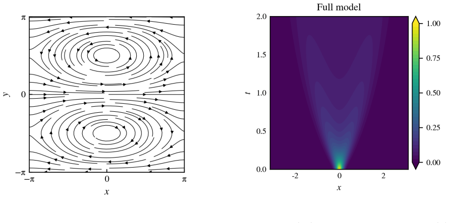
Example 1: Simple parallel flow We return to the caseu= cos(y). For this flow, the velocity-based variables are linear combinations of the spectral-based variables; thus, the two reduced model families are equiv- alent. Accordingly, we report only the results from spectral-based models. The evolution of the mean field ¯cfor this case has been shown in Fig...
-
[4]
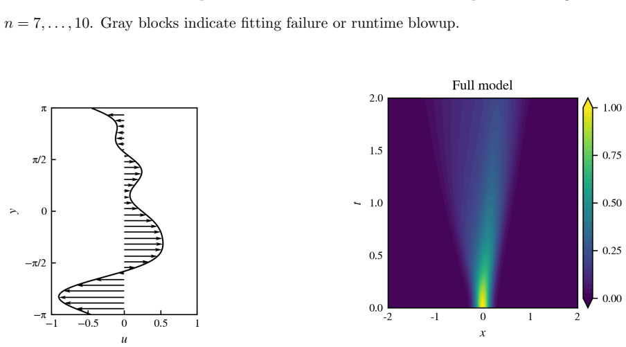
Example 2: Complex asymmetric parallel flow We next consider the more complex asymmetric shear flow profile in Eq. (78). The velocity profile and the time history of ¯cfor the test case are shown in Fig. 10. Further details of the full model solution are shown in Fig. 11. In contrast to the simple cosine shear flow case, ¯cis no longer symmetric inxdue to...
-
[5]
(59) following Ref
Problem statement We consider a two-dimensional unsteady inhomogeneous advection-diffusion problem, adapted from Eq. (59) following Ref. [11]: ∂c ∂t +u 1(x, y) ∂c ∂x +u 2(x, y) ∂c ∂y = 0.05 ∂2c ∂x2 + ∂2c ∂y 2 ,Ω = [−π, π]×[−π, π].(79) The system is periodic in bothxandy, with initial conditionc(x, y,0) = ¯c 0(x). The averaging operator ¯•denotes the cross...
-
[6]
Reduced variables and GFM forcing construction.Following the discussion in Sec
Numerical discovery of the reduced model a. Reduced variables and GFM forcing construction.Following the discussion in Sec. III B, we consider both spectral-based and velocity-based reduced variables. For the spectral-based variables, we adopt the cosine-mode definition in Eq. (69), motivated by the symmetry of the velocity field iny. For the velocity-bas...
-
[7]
(80) and (81), the eGFM training data are generated on a coarse grid withN x = 32,N y = 32, ∆t= 8×10 −3,T max = 8, and zero initial condition ¯c0 ≡0
Results and discussion For both inhomogeneous flow cases, Eqs. (80) and (81), the eGFM training data are generated on a coarse grid withN x = 32,N y = 32, ∆t= 8×10 −3,T max = 8, and zero initial condition ¯c0 ≡0. Compared to the example in Sec. III, more temporal snapshots are taken to improve the stability of the pointwise fit. For modeling, we consider ...
-
[8]
Problem statement We consider a modified version of Eq. (59) where the velocity carries a random temporal fluctuation: ∂c ∂t +u(y, t) ∂c ∂x = ∂2c ∂y 2 ,Ω = (−∞,∞)×[−π, π],(87) with periodic boundary conditions inyand initial conditionc(x, y,0) = ¯c 0(x). The velocity is given by u(y, t) = cos(y) 1 + 0.5β(t) ,(88) whereβ(t) is a zero-mean Gaussian process ...
-
[9]
Reduced variables and GFM forcing construction.As in Sec
Numerical discovery of the reduced model a. Reduced variables and GFM forcing construction.As in Sec. III B, we consider both spectral-based and velocity-based reduced variables. Sinceu(y, t) is symmetric iny, the spectral-based variables follow the cosine-mode definition in Eq. (69). The velocity-based variables follow Eq. (72). As discussed in Sec. III ...
-
[11]
Smagorinsky, General circulation experiments with the primitive equations: I
J. Smagorinsky, General circulation experiments with the primitive equations: I. the basic experiment, Monthly weather review91, 99 (1963)
1963
-
[12]
S. B. Pope, Turbulent flows, Measurement Science and Technology12, 2020 (2001)
2020
-
[13]
B. Sanderse, P. Stinis, R. Maulik, and S. E. Ahmed, Scientific machine learning for closure models in multiscale problems: A review, arXiv preprint arXiv:2403.02913 (2024)
-
[14]
Hamba, An analysis of nonlocal scalar transport in the convective boundary layer using the green’s function, Journal of Atmospheric Sciences52, 1084 (1995)
F. Hamba, An analysis of nonlocal scalar transport in the convective boundary layer using the green’s function, Journal of Atmospheric Sciences52, 1084 (1995)
1995
-
[15]
Hamba, Nonlocal expression for scalar flux in turbulent shear flow, Physics of Fluids16, 1493 (2004)
F. Hamba, Nonlocal expression for scalar flux in turbulent shear flow, Physics of Fluids16, 1493 (2004)
2004
-
[16]
Hamba, Nonlocal analysis of the reynolds stress in turbulent shear flow, Physics of Fluids 17(2005)
F. Hamba, Nonlocal analysis of the reynolds stress in turbulent shear flow, Physics of Fluids 17(2005)
2005
-
[17]
Hamba, Analysis and modelling of non-local eddy diffusivity for turbulent scalar flux, Journal of Fluid Mechanics950, A38 (2022)
F. Hamba, Analysis and modelling of non-local eddy diffusivity for turbulent scalar flux, Journal of Fluid Mechanics950, A38 (2022)
2022
-
[18]
Hamba, Analysis and modelling of non-local eddy diffusivity in turbulent channel flow, Journal of Fluid Mechanics1012, A21 (2025)
F. Hamba, Analysis and modelling of non-local eddy diffusivity in turbulent channel flow, Journal of Fluid Mechanics1012, A21 (2025)
2025
-
[19]
Hamba, Nonlocal eddy viscosity for reynolds stress and passive vector flux in turbulence, Physical Review Fluids10, 124601 (2025)
F. Hamba, Nonlocal eddy viscosity for reynolds stress and passive vector flux in turbulence, Physical Review Fluids10, 124601 (2025)
2025
-
[20]
Mani and D
A. Mani and D. Park, Macroscopic forcing method: a tool for turbulence modeling and analysis of closures, Physical Review Fluids6, 054607 (2021)
2021
-
[21]
J. Liu, H. H. Williams, and A. Mani, Systematic approach for modeling a nonlocal eddy diffusivity, Physical Review Fluids8, 124501 (2023)
2023
-
[22]
Park and A
D. Park and A. Mani, Direct calculation of the eddy viscosity operator in turbulent channel flow at reτ= 180, Journal of Fluid Mechanics998, A33 (2024). 48
2024
-
[23]
Lavacot, J
D.-L. Lavacot, J. Liu, H. Williams, B. E. Morgan, and A. Mani, Non-locality of mean scalar transport in two-dimensional rayleigh–taylor instability using the macroscopic forcing method, Journal of Fluid Mechanics985, A47 (2024)
2024
-
[24]
van der Oord, M
C. van der Oord, M. Sachs, D. P. Kov´ acs, C. Ortner, and G. Cs´ anyi, Hyperactive learning for data-driven interatomic potentials, npj Computational Materials9, 168 (2023)
2023
-
[25]
G. I. Taylor, Dispersion of soluble matter in solvent flowing slowly through a tube, Proceedings of the Royal Society of London. Series A. Mathematical and Physical Sciences219, 186 (1953)
1953
-
[26]
Aris, On the dispersion of a solute in a fluid flowing through a tube, Proceedings of the Royal Society of London
R. Aris, On the dispersion of a solute in a fluid flowing through a tube, Proceedings of the Royal Society of London. Series A. Mathematical and Physical Sciences235, 67 (1956)
1956
-
[27]
G. I. Taylor, Conditions under which dispersion of a solute in a stream of solvent can be used to measure molecular diffusion, Proceedings of the Royal Society of London. Series A. Mathematical and Physical Sciences225, 473 (1954)
1954
-
[28]
Gill and R
W. Gill and R. Sankarasubramanian, Exact analysis of unsteady convective diffusion, Pro- ceedings of the Royal Society of London. A. Mathematical and Physical Sciences316, 341 (1970)
1970
-
[29]
Barton, On the method of moments for solute dispersion, Journal of Fluid Mechanics126, 205 (1983)
N. Barton, On the method of moments for solute dispersion, Journal of Fluid Mechanics126, 205 (1983)
1983
-
[30]
Frankel and H
I. Frankel and H. Brenner, On the foundations of generalized taylor dispersion theory, Journal of Fluid Mechanics204, 97 (1989)
1989
-
[31]
Moyal, Stochastic processes and statistical physics, Journal of the Royal Statistical Society
J. Moyal, Stochastic processes and statistical physics, Journal of the Royal Statistical Society. Series B (Methodological)11, 150 (1949)
1949
-
[32]
Virtanen, R
P. Virtanen, R. Gommers, T. E. Oliphant, M. Haberland, T. Reddy, D. Cournapeau, E. Burovski, P. Peterson, W. Weckesser, J. Bright,et al., Scipy 1.0: fundamental algorithms for scientific computing in python, Nature methods17, 261 (2020)
2020
-
[33]
Frigo and S
M. Frigo and S. G. Johnson, The design and implementation of fftw3, Proceedings of the IEEE 93, 216 (2005)
2005
-
[34]
Canuto, M
C. Canuto, M. Y. Hussaini, A. Quarteroni, and T. A. Zang,Spectral methods: fundamentals in single domains(Springer, 2006)
2006
-
[35]
C. L. Lawson and R. J. Hanson,Solving least squares problems(SIAM, 1995)
1995
-
[36]
Kubo, Stochastic liouville equations, Journal of Mathematical Physics4, 174 (1963)
R. Kubo, Stochastic liouville equations, Journal of Mathematical Physics4, 174 (1963). 49
1963
-
[37]
Mori, Transport, collective motion, and brownian motion, Progress of theoretical physics 33, 423 (1965)
H. Mori, Transport, collective motion, and brownian motion, Progress of theoretical physics 33, 423 (1965)
1965
-
[38]
W. Xue and A. Mani, Reproduction data and scripts for “Generalized Forcing Method: Generation of Diverse Data for Training Linear Transport PDE Closure Models” (2026), https://doi.org/10.5281/zenodo.20424795. 50
This paper was first reviewed by grok-4.3 on June 28, 2026.
discussion (0)
Sign in with ORCID, Apple, or X to comment. Anyone can read and Pith papers without signing in.