Scaling Laws for Behavioral Foundation Models over User Event Sequences
Pith reviewed 2026-06-28 06:46 UTC · model grok-4.3
The pith
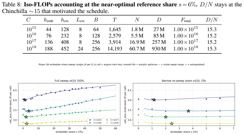
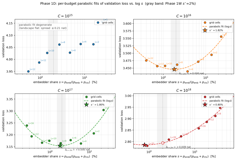
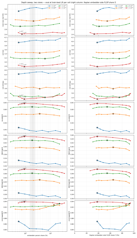
A small embedder of about 2% of parameters is compute-optimal at every budget for behavioral foundation models on user event sequences.
A machine-rendered reading of the paper's core claim, the machinery that carries it, and where it could break.
Core claim
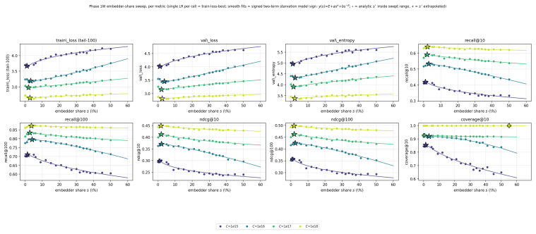
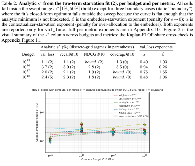
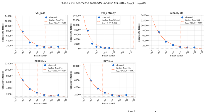
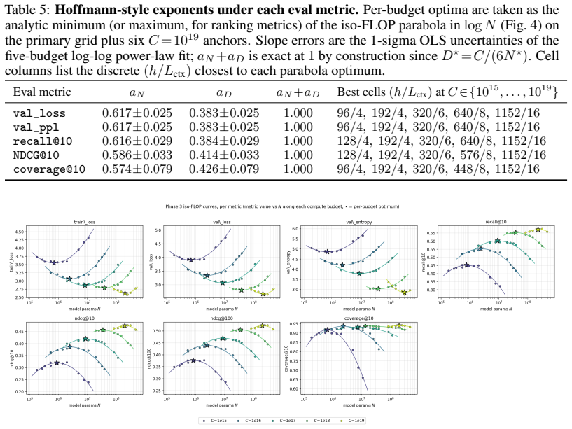
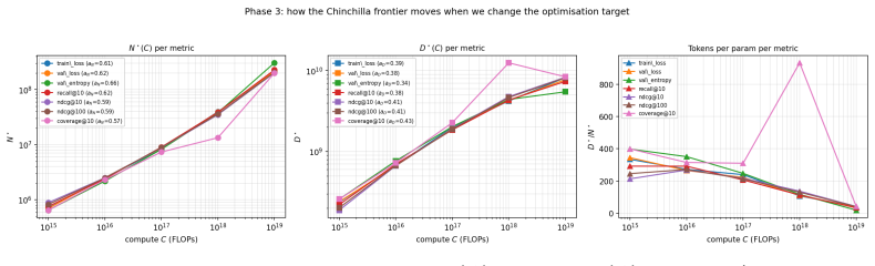
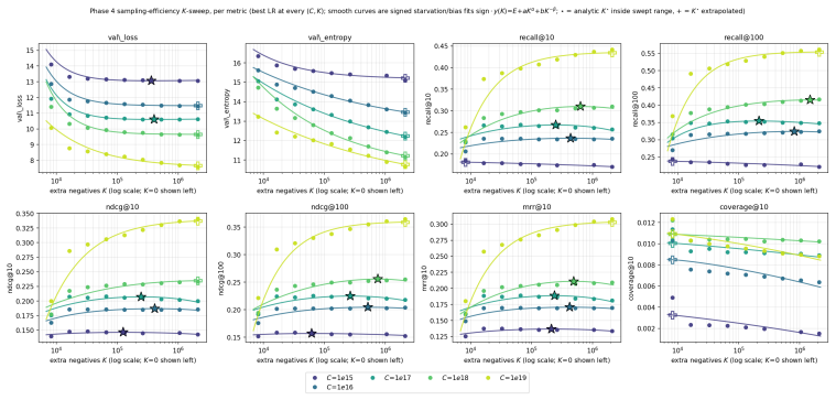
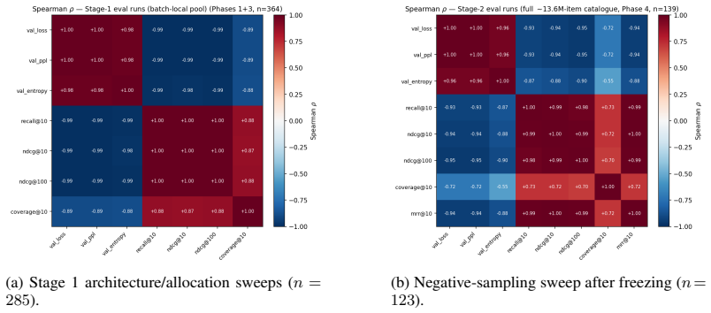
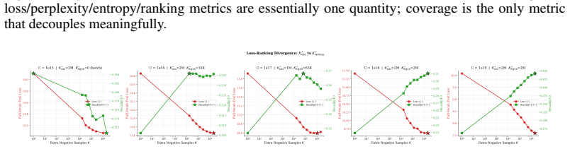
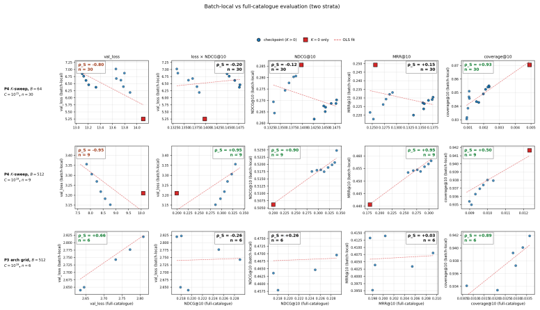
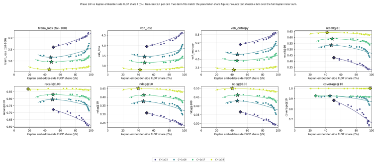
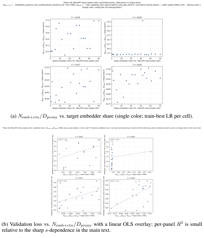
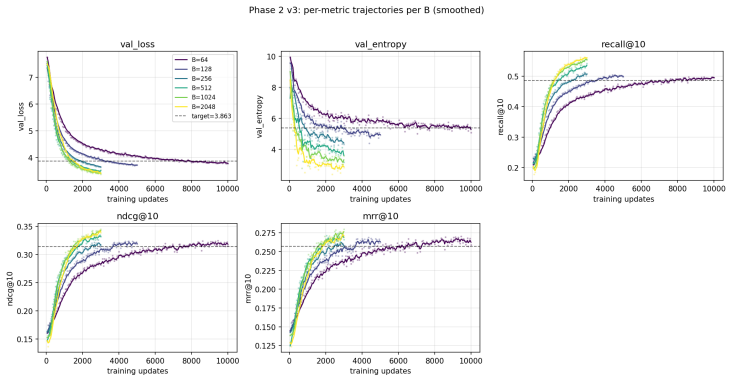
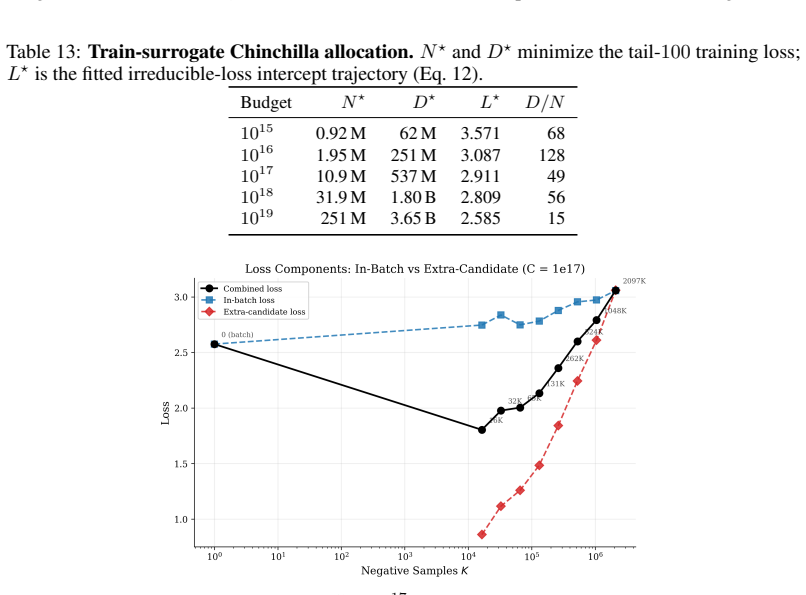
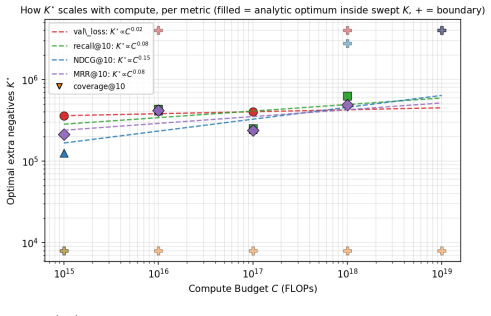
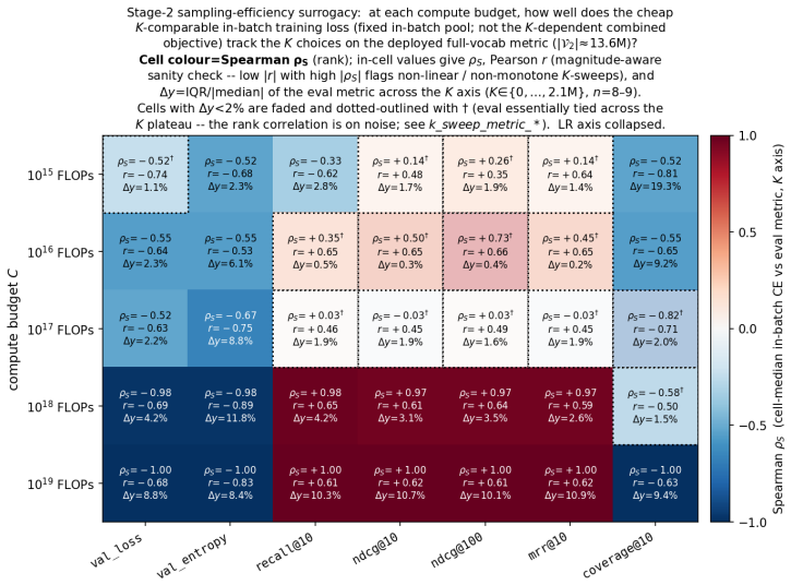
Across 600 runs on real interaction data from 10^15 to 10^19 FLOPs, the optimal embedder size s* is approximately 2% of total parameters at every compute budget. Embedder parameters are more expensive per training step and are exposed to far more repeated items than the contextualizer parameters. As a result, compute-optimal training starts data-heavy relative to language models but the D/N ratio approaches the Chinchilla heuristic at higher compute. The sampled training objective and ranking metrics disagree in ways that scale with compute and metric choice, with larger budgets preferring more negatives until memory limits are hit.
What carries the argument
The parameter split between the feature-based event embedder and the decoder-only transformer, which determines the optimal allocation because of differing per-step costs and repetition rates.
If this is right
- Embedder size should stay small even as total model size grows.
- Data allocation should be larger relative to parameters at smaller compute budgets.
- Negative sample count should increase with scale until candidate memory becomes the bottleneck.
- The choice of ranking metric affects the optimal training configuration.
- Scaling laws for these models must incorporate the evaluation metric as a variable.
Where Pith is reading between the lines
- Production systems could use this to allocate fewer parameters to embeddings and reduce overall training cost.
- Similar scaling might hold for other sequence models with high item repetition.
- Future work could test if unifying the embedder and contextualizer changes the optimal split.
- Disagreement scaling suggests loss functions may need to be adjusted or combined with ranking objectives at large scales.
Load-bearing premise
The trends in optimal embedder fraction and scaling behaviors will continue to hold outside the specific real interaction datasets and two-part architecture used in the experiments.
What would settle it
A new set of scaling runs on different user event data or with a different architecture showing that the optimal embedder fraction changes substantially with compute budget or is not around 2%.
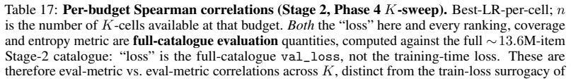
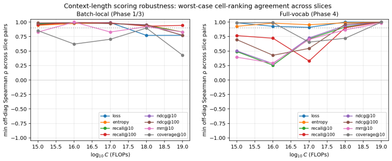
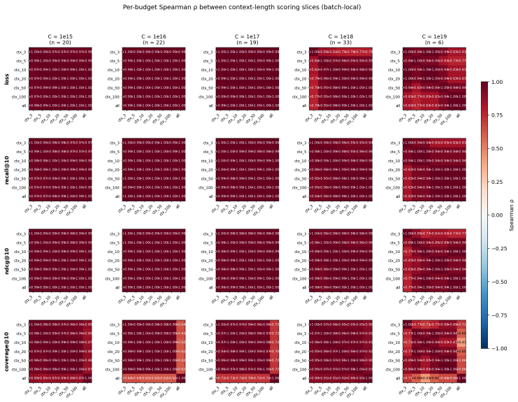
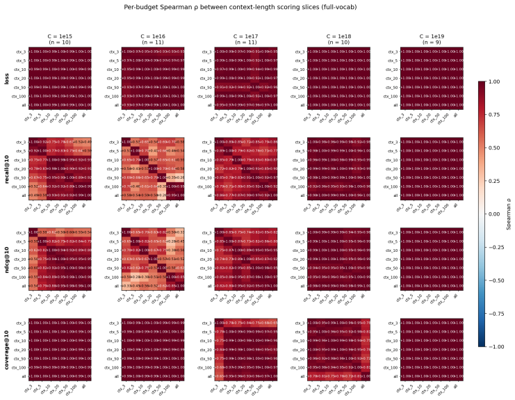
Figures

read the original abstract
Foundation models are increasingly trained on sequences of user actions in recommendation, payments, fraud, and commerce, but these models still lack the kind of compute calibration that scaling laws provide for language models. We study a common two-part behavioral-model architecture: a feature-based event embedder maps each multi-modal item to a vector, and a decoder-only transformer predicts the next event from the resulting sequence. Across roughly 600 runs on real interaction data, spanning $10^{15}$-$10^{19}$ training FLOPs, we jointly vary four deployment-relevant axes: the two-part parameter split, critical batch size, model/data allocation, and the number of sampled negatives used after freezing the embedder. A small embedder ($s^{\star}\!\approx\!2\%$ of parameters) is compute-optimal at every budget we test because embedder parameters are both more expensive per step and exposed to far more repeated items than contextualizer parameters. Compute-optimal training is data-heavy relative to text at low compute, but its $D/N$ ratio moves toward the Chinchilla heuristic as compute increases. The sampled training objective and deployed ranking metrics disagree in ways that themselves scale: critical batch size, optimal negative count after freezing, and the agreement between loss and ranking quality all shift with compute and with the chosen evaluation metric. For negative sampling, larger budgets increasingly prefer more negatives; by $10^{19}$ FLOPs the active constraint is candidate-axis memory rather than FLOPs. In behavioral foundation models, the evaluation metric is therefore part of the scaling law: changing it can change the compute-optimal recipe.
Editorial analysis
A structured set of objections, weighed in public.
Referee Report
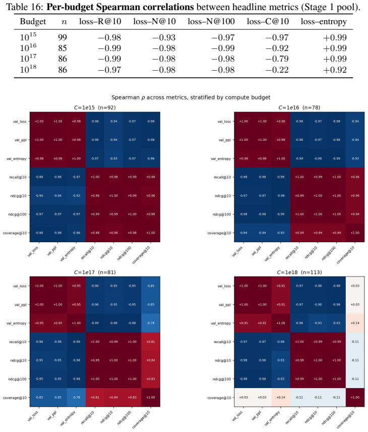
Summary. The paper claims that for two-part behavioral foundation models (feature-based event embedder + decoder-only transformer) trained on user event sequences, a small embedder fraction s* ≈ 2% of total parameters is compute-optimal across all tested budgets from 10^15 to 10^19 FLOPs. This is attributed to embedder parameters being more expensive per step and exposed to more repeated items. The work also reports that compute-optimal D/N ratios start data-heavy relative to Chinchilla but approach it at higher compute, that critical batch size and optimal negative count after freezing shift with scale, and that sampled loss and ranking metrics disagree in ways that themselves scale with compute and metric choice. These conclusions rest on ~600 runs on real interaction datasets jointly varying parameter split, batch size, model/data allocation, and negative count.
Significance. If the central empirical trends hold, the paper supplies the first large-scale compute-optimal calibration for behavioral models on event sequences, directly relevant to recommendation, payments, and fraud domains. The scale of the experimental campaign (600 runs spanning five orders of magnitude in FLOPs) is a clear strength and provides substantial empirical support for the observed trends in embedder fraction and negative-sampling preferences.
major comments (2)
- [Abstract] Abstract: the explanatory claim that s* ≈ 2% optimality arises 'because embedder parameters are both more expensive per step and exposed to far more repeated items than contextualizer parameters' is load-bearing for the interpretation. All 600 runs use real interaction datasets that exhibit high item repetition; the manuscript reports no controlled experiments that vary repetition rate (e.g., synthetic data with adjustable Zipf exponents) while holding other factors fixed, leaving open the possibility that the observed optimum is an artifact of the repetition statistics rather than a general architectural property.
- [Abstract] Abstract and experimental description: the 2% optimality claim and the scaling trends for critical batch size and negative count lack reported error bars, statistical significance tests for the 2% figure, explicit data-exclusion rules, or analysis of whether post-hoc metric choices affect the central trends. These omissions make it difficult to assess robustness of the reported optima.
minor comments (1)
- [Abstract] Abstract: the symbol s* is used before any definition or parenthetical explanation; a brief inline clarification would improve readability for readers encountering the abstract first.
Simulated Author's Rebuttal
We thank the referee for the constructive review and detailed comments. We address each major point below, indicating planned revisions where appropriate.
read point-by-point responses
-
Referee: [Abstract] Abstract: the explanatory claim that s* ≈ 2% optimality arises 'because embedder parameters are both more expensive per step and exposed to far more repeated items than contextualizer parameters' is load-bearing for the interpretation. All 600 runs use real interaction datasets that exhibit high item repetition; the manuscript reports no controlled experiments that vary repetition rate (e.g., synthetic data with adjustable Zipf exponents) while holding other factors fixed, leaving open the possibility that the observed optimum is an artifact of the repetition statistics rather than a general architectural property.
Authors: We agree that our experiments are confined to real interaction datasets exhibiting high item repetition and that we did not perform controlled synthetic experiments varying repetition rates (e.g., via adjustable Zipf exponents). The 2% optimum and its proposed mechanism are therefore tied to the statistical properties of the real data used. While the trend is consistent across multiple distinct real-world datasets, this does not fully rule out dataset-specific artifacts. We will revise the abstract and discussion sections to present the explanation as a hypothesis grounded in architectural differences and observed repetition patterns in behavioral data, rather than a proven general causal factor, and will explicitly note the lack of synthetic controls as a limitation. revision: partial
-
Referee: [Abstract] Abstract and experimental description: the 2% optimality claim and the scaling trends for critical batch size and negative count lack reported error bars, statistical significance tests for the 2% figure, explicit data-exclusion rules, or analysis of whether post-hoc metric choices affect the central trends. These omissions make it difficult to assess robustness of the reported optima.
Authors: We acknowledge these gaps in the current version. In revision we will add error bars (computed from replicate runs where available) to all figures reporting the 2% optimum and scaling trends for batch size and negative count. We will include statistical significance tests for the identified optima. Data-exclusion criteria (based on convergence thresholds and outlier detection) will be stated explicitly in the experimental section. We will also add an analysis of how the central trends vary with different post-hoc metric choices and report the sensitivity of the scaling conclusions to metric selection. revision: yes
Circularity Check
No circularity; results are direct empirical observations from 600 runs
full rationale
The paper presents scaling trends as outcomes of joint variation across four axes in ~600 real-data training runs spanning 10^15 to 10^19 FLOPs. Optimal embedder fraction s*≈2%, D/N ratios, negative counts, and metric disagreements are reported as measured quantities rather than quantities derived from equations that reduce to the inputs by construction. No self-definitional steps, fitted-input predictions, or load-bearing self-citations appear in the provided text; the 'because' clause in the abstract is an interpretive summary of the observed trends, not a mathematical reduction.
Axiom & Free-Parameter Ledger
free parameters (1)
- optimal embedder fraction s* =
0.02
axioms (1)
- domain assumption The two-part feature-based embedder plus decoder-only transformer is a suitable architecture for modeling user event sequences.
Reference graph
Works this paper leans on
-
[1]
Scaling Laws for Neural Language Models
J. Kaplan et al. Scaling laws for neural language models.arXiv:2001.08361, 2020
work page internal anchor Pith review Pith/arXiv arXiv 2001
-
[2]
Training Compute-Optimal Large Language Models
J. Hoffmann et al. Training compute-optimal large language models (Chinchilla). arXiv:2203.15556, 2022
work page internal anchor Pith review Pith/arXiv arXiv 2022
-
[3]
Yang and E
G. Yang and E. Hu. Tensor Programs IV: Feature learning in infinite-width neural networks (MuP). InICML, 2021
2021
-
[4]
An Empirical Model of Large-Batch Training
S. McCandlish, J. Kaplan, D. Amodei, and the OpenAI Dota Team. An empirical model of large-batch training.arXiv:1812.06162, 2018
work page internal anchor Pith review Pith/arXiv arXiv 2018
-
[5]
Zhai et al
J. Zhai et al. Actions speak louder than words: Trillion-parameter sequential transducers for generative recommendations (HSTU). InICML, 2024. 16
2024
-
[6]
B. Zhang et al. Wukong: Towards a scaling law for large-scale recommendation. arXiv:2403.02545, 2024
-
[7]
N. Ardalani et al. Understanding scaling laws for recommendation models.arXiv:2208.08489, 2022
-
[8]
H. Liu, C. Li, Q. Wu, and Y . J. Lee. Visual instruction tuning. InNeurIPS, 2023
2023
-
[9]
Alayrac et al
J.-B. Alayrac et al. Flamingo: a visual language model for few-shot learning. InNeurIPS, 2022
2022
-
[10]
J. Li, D. Li, S. Savarese, and S. Hoi. BLIP-2: Bootstrapping language-image pre-training with frozen image encoders and large language models. InICML, 2023
2023
-
[11]
Covington, J
P. Covington, J. Adams, and E. Sargin. Deep neural networks for YouTube recommendations. InACM RecSys, 2016
2016
-
[12]
Bengio and J.-S
Y . Bengio and J.-S. Senécal. Adaptive importance sampling to accelerate training of a neural probabilistic language model.IEEE Transactions on Neural Networks, 19(4):713–722, 2008
2008
-
[13]
Foundation Model for Personalized Recommendation
Netflix Technology Blog. Foundation Model for Personalized Recommendation. Mar. 2025. https://netflixtechblog.com/ foundation-model-for-personalized-recommendation-1a0bd8e02d39
2025
-
[14]
C.-C. M. Yeh, U. S. Saini, X. Dai, X. Fan, S. Jain et al. TREASURE: A transformer-based foundation model for high-volume transaction understanding (Visa Payment Foundation Model). arXiv:2511.19693, 2025
work page internal anchor Pith review Pith/arXiv arXiv 2025
- [15]
-
[16]
Kedia and the Stripe Machine Learning Team
G. Kedia and the Stripe Machine Learning Team. Stripe’s Payments Foundation Model. Stripe Sessions / Stripe Engineering, May 2025
2025
-
[17]
PRAGMA: Revolut Foundation Model
V . Iashin et al. PRAGMA: Revolut foundation model.arXiv:2604.08649, 2026
work page internal anchor Pith review Pith/arXiv arXiv 2026
-
[18]
M. Kawawa-Beaudan, D. Borrajo, M. Veloso et al. TradeFM: A generative foundation model for trade-flow and market microstructure.arXiv:2602.23784, 2026
-
[19]
Brüel Gabrielsson et al
R. Brüel Gabrielsson et al. A foundation model for consumption, transactions, and actions: The inception of BehaviorGPT. Unbox AI Research, 2025
2025
-
[20]
Brüel Gabrielsson and V
R. Brüel Gabrielsson and V . Gupta. BehaviorGPT at work: A foundation model for workforce actions and dynamics. Unbox AI Research, 2025
2025
-
[21]
Brüel Gabrielsson and V
R. Brüel Gabrielsson and V . Gupta. BehaviorGPT for visual art: A foundation model for aesthetics. Unbox AI Research, 2025
2025
-
[22]
Brüel Gabrielsson et al
R. Brüel Gabrielsson et al. Large behavioral models: A foundation-model paradigm for human actions. Unbox AI Research, 2026
2026
-
[23]
Järvelin and J
K. Järvelin and J. Kekäläinen. Cumulated gain-based evaluation of IR techniques.ACM Transactions on Information Systems, 20(4):422–446, 2002
2002
-
[24]
E. M. V oorhees. The TREC-8 question answering track report. InProceedings of TREC-8, 1999
1999
-
[25]
C. D. Manning, P. Raghavan, and H. Schütze.Introduction to Information Retrieval. Cambridge University Press, 2008
2008
-
[26]
J. L. Herlocker, J. A. Konstan, L. G. Terveen, and J. T. Riedl. Evaluating collaborative filtering recommender systems.ACM Transactions on Information Systems, 22(1):5–53, 2004. 17 A Metric Definitions Notation and candidate set.Every metric scores each query position against acandidate set C and ranks its items by the dot-product score zq,j =⟨h q, ej⟩, w...
discussion (0)
Sign in with ORCID, Apple, or X to comment. Anyone can read and Pith papers without signing in.