Setting angles in quantum approximate optimization at utility-scale
Pith reviewed 2026-06-28 05:34 UTC · model grok-4.3
The pith
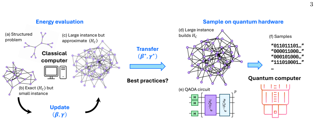
QAOA angles trained on small problems transfer effectively to utility-scale hardware instances.
A machine-rendered reading of the paper's core claim, the machinery that carries it, and where it could break.
Core claim
Utility-scale benchmarks show that angles obtained by training on small representative problems and then transferred to larger instances achieve competitive performance on hardware-executable problems, while approximation techniques such as matrix product states and Pauli propagation offer alternative routes whose quality depends on the computational resources allocated to the angle search.
What carries the argument
Angle transfer from small-scale representative problems combined with matrix-product-state and Pauli-propagation approximations, validated through direct hardware execution on executable utility-scale instances.
If this is right
- Practitioners can avoid full-scale classical optimization by using transferred angles when resource budgets are limited.
- Approximation methods become viable substitutes once their accuracy-cost curve is known for the target problem class.
- Hardware-executable utility-scale instances serve as the decisive testbed for any proposed angle-setting rule.
- End-to-end QAOA pipelines become feasible on current hardware by matching the angle method to the available classical compute.
Where Pith is reading between the lines
- The same transfer principle may apply to other variational quantum algorithms that use layered parameterized circuits.
- If small-problem similarity holds, it reduces the need to simulate or optimize at full scale before hardware execution.
- Noise on real hardware may alter which angle-setting method is optimal compared with ideal simulations.
Load-bearing premise
Small-scale problems are similar enough to utility-scale instances that angles found on the former remain useful on the latter.
What would settle it
Direct measurement on hardware showing that transferred angles produce markedly lower approximation ratios than angles obtained by optimizing the large instance itself.
Figures

read the original abstract
The quantum approximate optimization algorithm (QAOA) is a powerful heuristic that seeks to solve combinatorial optimization problems using quantum hardware and classical optimization in tandem. Various methods exist to train the parameterized quantum circuits that serve as an ansatz in QAOA. However, which method works best to identify optimal angles for a given problem instance remains poorly understood, especially at utility-scale, i.e., $100$ qubits or more. In this work, we address this challenge through utility-scale benchmarks from which we distill operational guidance for QAOA practitioners. First, we investigate approximation techniques, such as matrix product states and Pauli propagation, to find optimal angles. Second, we train QAOA on small-scale representative problems and transfer the angles to larger ones. We then validate the results on quantum hardware for utility-scale problem instances that can be meaningfully executed. In this way, we identify insights for QAOA angle setting strategies that work best for problems at the utility scale, including as a function of resource cost for the search. Crucially, the operational implications we draw from our benchmarks will help quantum optimization practitioners execute QAOA end-to-end pipelines efficiently on current and future hardware.
Editorial analysis
A structured set of objections, weighed in public.
Referee Report
Summary. The paper benchmarks QAOA angle-setting methods at utility scale (≥100 qubits), comparing approximation techniques such as matrix product states and Pauli propagation against training on small representative instances followed by angle transfer, with hardware validation restricted to 'meaningfully executable' utility-scale cases; from these benchmarks the authors distill operational guidance on which strategies perform best as a function of search resource cost.
Significance. If the empirical comparisons are robust, the work supplies concrete, resource-aware recommendations that could improve end-to-end QAOA pipelines on present-day hardware; the explicit focus on transferability and hardware-executable instances is a practical strength.
major comments (3)
- [Abstract and §4] Abstract and §4 (Results): the central claim that transferred angles yield reliable operational guidance at utility scale rests on the untested premise that optimal angles (or their ranking) are insensitive to system size; the manuscript provides no quantitative comparison of the transfer gap (e.g., energy or approximation-ratio difference between small-scale optima and large-scale performance) nor any scaling study of landscape features with n.
- [§3.2] §3.2 (Instance selection): restricting hardware validation to 'meaningfully executable' utility-scale instances introduces a selection bias; the paper does not demonstrate that these instances are representative of the broader class of problems for which transfer is claimed to work, nor does it report how many candidate instances were discarded and why.
- [§5] §5 (Discussion of insights): the distilled 'insights' are presented without error bars, statistical significance tests across instances, or ablation of the approximation methods (MPS vs. Pauli propagation) against a simple baseline such as random or fixed-angle initialization; this weakens the claim that the benchmarks support actionable guidance.
minor comments (2)
- [Notation] Notation for the number of layers p and the cost/resource metrics is introduced inconsistently between the abstract and the methods section; a single table of symbols would improve clarity.
- [Figures] Figure captions for the hardware results do not state the number of shots, the error-mitigation protocol, or the precise definition of 'meaningfully executed,' making the plots hard to interpret without the main text.
Simulated Author's Rebuttal
We thank the referee for the constructive and detailed comments. We have revised the manuscript to address the concerns regarding the transfer premise, instance selection transparency, and statistical rigor in the insights. Below we respond point-by-point.
read point-by-point responses
-
Referee: [Abstract and §4] Abstract and §4 (Results): the central claim that transferred angles yield reliable operational guidance at utility scale rests on the untested premise that optimal angles (or their ranking) are insensitive to system size; the manuscript provides no quantitative comparison of the transfer gap (e.g., energy or approximation-ratio difference between small-scale optima and large-scale performance) nor any scaling study of landscape features with n.
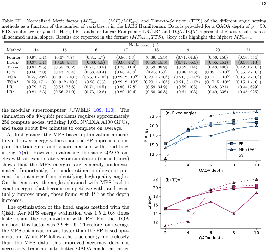
Authors: We acknowledge that a direct scaling study of landscape features and a full quantification of the transfer gap (difference between small-scale optima and large-scale performance) would provide stronger support. Our hardware validation on utility-scale instances measures the practical end-to-end performance of transferred angles, which forms the basis for the operational guidance. In the revised manuscript we have added a quantitative discussion in §4 of the observed approximation-ratio differences between transferred angles and small-scale optima (where direct optimization at large scale is infeasible), along with a note that a comprehensive scaling analysis of the QAOA landscape remains an important open direction. (partial) revision: partial
-
Referee: [§3.2] §3.2 (Instance selection): restricting hardware validation to 'meaningfully executable' utility-scale instances introduces a selection bias; the paper does not demonstrate that these instances are representative of the broader class of problems for which transfer is claimed to work, nor does it report how many candidate instances were discarded and why.
Authors: We agree that transparency on the selection process is necessary. The revised §3.2 now reports the total number of candidate utility-scale instances initially generated, the precise definition of 'meaningfully executable' (circuit depth and estimated noise thresholds compatible with current hardware), the number of instances discarded, and the reasons for exclusion. We further argue representativeness by showing that the retained instances span the same range of problem densities and graph structures as the broader ensemble used for the transfer-learning benchmarks. (yes) revision: yes
-
Referee: [§5] §5 (Discussion of insights): the distilled 'insights' are presented without error bars, statistical significance tests across instances, or ablation of the approximation methods (MPS vs. Pauli propagation) against a simple baseline such as random or fixed-angle initialization; this weakens the claim that the benchmarks support actionable guidance.
Authors: The referee is correct that additional statistical controls would strengthen the claims. In the revised §5 we now report error bars on all averaged metrics (computed over the instance ensemble), include paired statistical significance tests comparing the methods, and add an ablation against random-angle and fixed-angle (p=0.5) baselines. These updates make the operational guidance more robustly supported by the data. (yes) revision: yes
Circularity Check
Empirical benchmarking with no derivation chain
full rationale
The paper presents an empirical study: it benchmarks approximation techniques (MPS, Pauli propagation) for angle optimization, trains on small instances and transfers angles to larger ones, then validates on hardware-executable utility-scale cases. No mathematical derivation, first-principles result, or parameter fit is claimed to predict a distinct quantity; the work explicitly frames itself as distilling operational guidance from benchmarks. No self-citations are invoked as load-bearing uniqueness theorems, no ansatz is smuggled, and no quantity is renamed as a new result. The central claims rest on experimental outcomes rather than any reduction to inputs by construction, satisfying the criteria for a self-contained empirical paper.
Axiom & Free-Parameter Ledger
Forward citations
Cited by 1 Pith paper
-
Feasibility-driven QAOA with penalty scheduling
Introduces Λ-lr-QAOA and piecewise-ramp QAOA that promote penalty schedules to variational parameters and use a feasibility-driven loss on budget-constrained MWIS satellite planning instances.
Reference graph
Works this paper leans on
-
[1]
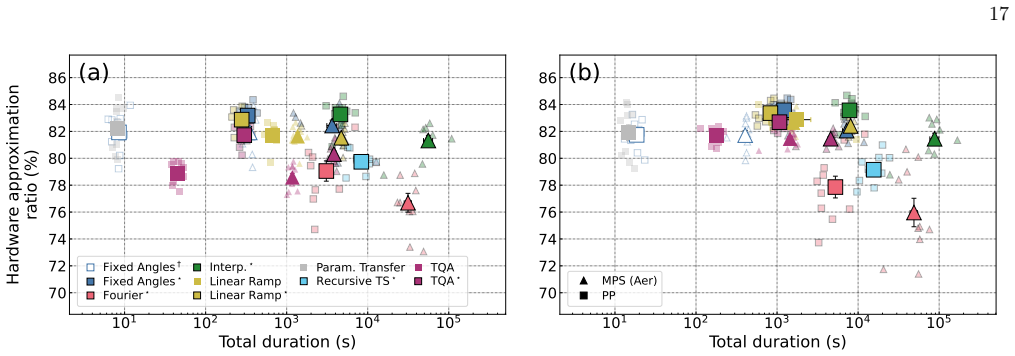
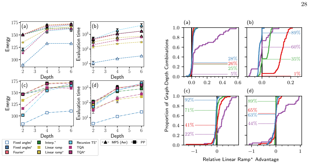
VB of the main text, we transfer angles from small-scale heavy-hex and line-based problems to larger ones
Parameter transfer In Sec. VB of the main text, we transfer angles from small-scale heavy-hex and line-based problems to larger ones. The parameter transfer is done as follows. (i) We construct a database of optimized QAOA angles contain- ing 12 and 39 nodes heavy-hex graphs and line-based graphs with 10 to 22 nodes. The QAOA angles for the ≤22and 39 node...
-
[2]
For a given depthp, QAOA-PCA requires a training set of precomputed optimal angles forNdiffer- ent problem instances, given as anN×2pmatrixX
Principal Component QAOA Inspired by clustering and transferability observa- tions [39, 116], QAOA-PCA [53] uses principle compo- nent analysis to reduce the dimensionality of the QAOA angle space. For a given depthp, QAOA-PCA requires a training set of precomputed optimal angles forNdiffer- ent problem instances, given as anN×2pmatrixX. The 2p×2pcovarian...
2000
-
[3]
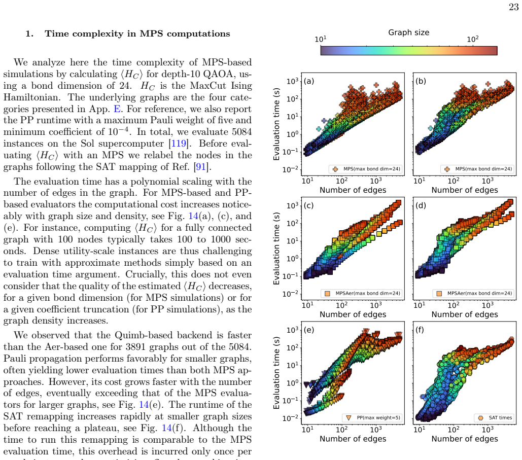
The underlying graphs are the four cate- gories presented in App
Time complexity in MPS computations We analyze here the time complexity of MPS-based simulations by calculating⟨HC⟩for depth-10 QAOA, us- ing a bond dimension of 24.H C is the MaxCut Ising Hamiltonian. The underlying graphs are the four cate- gories presented in App. E. For reference, we also report the PP runtime with a maximum Pauli weight of five and m...
-
[4]
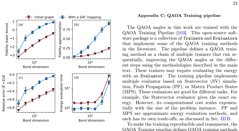
[29] to gauge the accuracy of an MPS-based simulation
Fidelity bounds in MPS computations We now show two metrics from Ref. [29] to gauge the accuracy of an MPS-based simulation. The first metric Fbound = 1−2 NgX i=1 vuut1− mX j=1 λ2 j,i ,(B1) lower-bounds the fidelity of the simulation [29]. Here, Ng is the number of two-qubit gates of the circuit,m is the bond dimension, and{λj,i}m j=1 are themsingular val...
-
[5]
For loop-free TNs (such as MPS) efficient methods for executing both steps exists [120], with a computational cost scaling polynomially with the bond dimension
Sampling and energy evaluation For a given TN state|ΨTN⟩, calculating the average of an operator⟨Ψ TN|O|ΨTN⟩and sampling from the probability distributionp σ =|⟨σ|Ψ TN⟩|2 do not have the same complexity. For loop-free TNs (such as MPS) efficient methods for executing both steps exists [120], with a computational cost scaling polynomially with the bond dim...
-
[6]
Goemans-Williamson as a baseline A genuinely challenging baseline for QAOA to beat on MaxCut is the Goemans-Williamson algorithm [6], which is fully classical and runs in polynomial-time. For the heavy-hex, Erdős-Rényi, random-regular, and line-based instances considered throughout the paper, we gener- ate results for 10, 100, 1000, and 10000 rounds of th...
-
[7]
VA obtained with state vectors for small-scale instances, i.e.n≤22nodes
Statevector results In this section we show a deeper analysis of the results in Sec. VA obtained with state vectors for small-scale instances, i.e.n≤22nodes. The approximation ratio of MaxCutforErdős-Rényi, random-regular, andline-based graphs steadily increases with depthp, see Fig. 16(a). The density and the average node degree of the graphs included in...
-
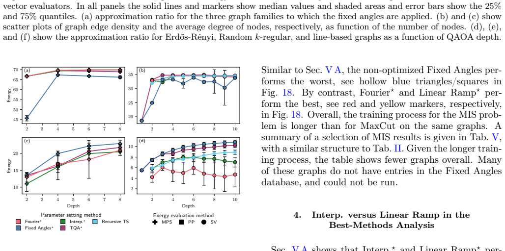
[8]
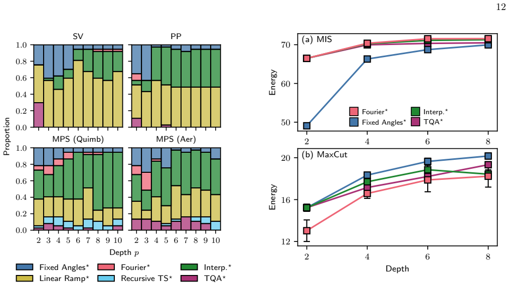
Additional MIS and MaxCut data Here, we first present results with MPS and Statevec- tor energy evaluation for MIS and MaxCut problems based on three-regular graphs, complementing the PP data shown in Sec. VA. MPS have a similar behavior to the PP results shown in Sec. VA. Fourier⋆ is best in terms of energy for MIS, and the Fixed Angles⋆ is best for MaxC...
-
[9]
versus Linear Ramp in the Best-Methods Analysis Sec
Interp. versus Linear Ramp in the Best-Methods Analysis Sec. VA shows that Interp.⋆ and Linear Ramp⋆ per- form well across all energy evaluation methods and depths, when run on the37-graph dataset. In particular, Interp.⋆ appears better with MPS whereas Linear Ramp⋆ is better with SV. The split is approximately “50/50” for PP. Here we analyze the differen...
1920
-
[10]
D, is a notoriously difficult combinatorial optimization problem even at small sizes
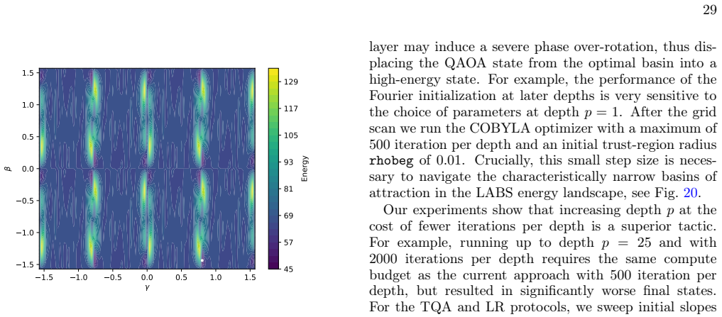
LABS LABS, defined in App. D, is a notoriously difficult combinatorial optimization problem even at small sizes. The cost landscape is extremely rugged; single spin-flips in a near-optimal sequence typically degrade the en- ergy to values indistinguishable from the ensemble aver- age [106, 107]. The classical state of the art exact solver 0.0 0.2 0.4 0.6 ...
2000
-
[11]
Theyarebasedonsuperconductingqubitquantum processing units (QPU) with a heavy-hexagonal qubit coupling topology
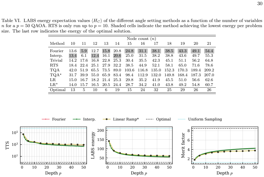
Quantum circuit creation Our hardware experiments run on IBM Quantum de- vices. Theyarebasedonsuperconductingqubitquantum processing units (QPU) with a heavy-hexagonal qubit coupling topology. The native gate set is built from 30 Table VI. LABS energy expectation values⟨HC ⟩of the different angle setting methods as a function of the number of variables nf...
-
[12]
T raining QAOA angles on hardware Here, we provide details on the hardware training ex- ample of Sec. IIIB1. The graph considered is built from a line of 100 nodes on which two layers of SWAP gates are applied. Each edge is assigned a weight of±1with 50%probability. We use COBYLA to minimize⟨H C⟩α computed over theα= 5%best samples ranked by the MaxCut ob...
1980
-
[13]
An efficient and exact computation of the depth- one energy, shown in Fig
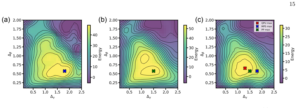
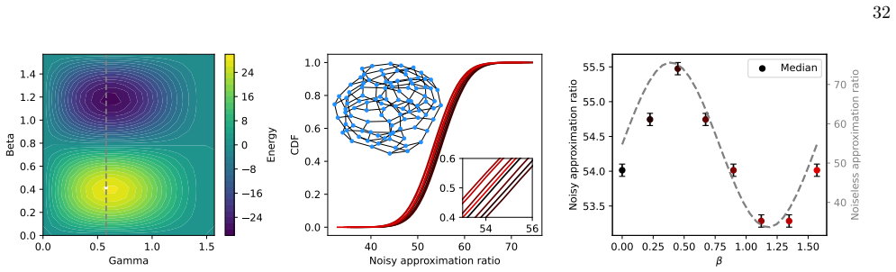
Angle validation Here, we further exemplify the quantum hardware val- idation by evaluating the energy on a QPU of a depth- one QAOA for a random three-regular graph with 100 nodes. An efficient and exact computation of the depth- one energy, shown in Fig. 22(a), serves as a ground truth. We create a hardware-native QAOA circuit with SWAP networks and a S...
-
[14]
VB are statistically meaningful
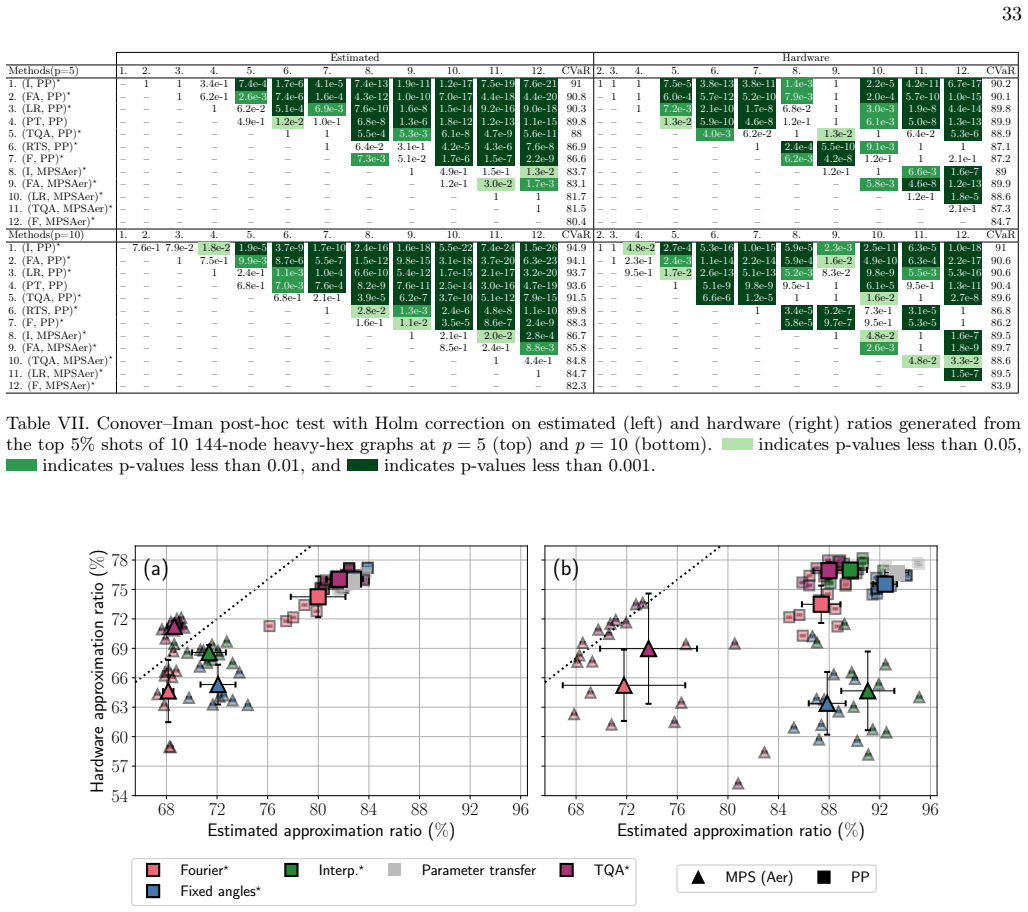
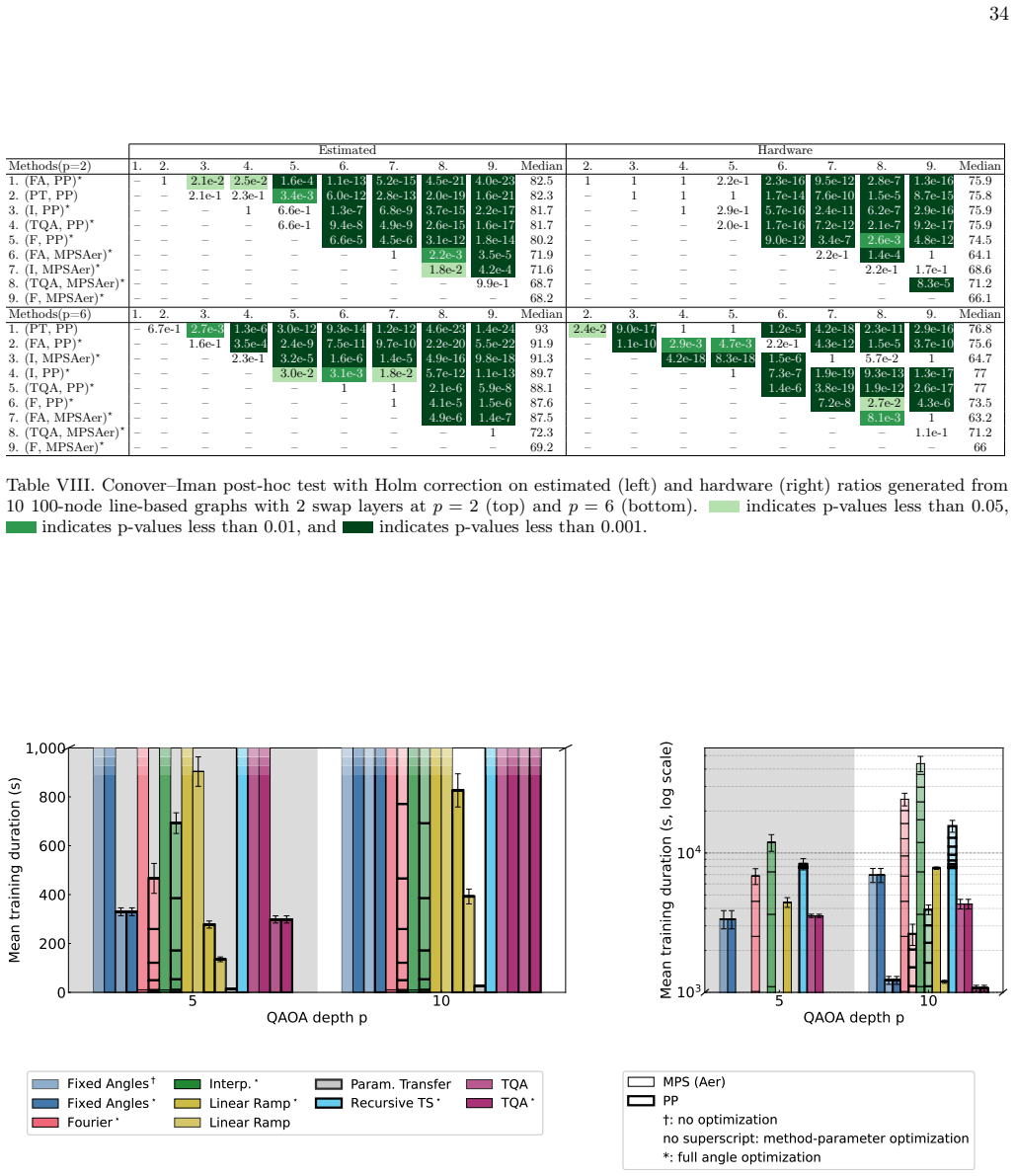
Statistical analysis Here, we describe the analysis used to determine whether the differences between the approximation ra- tios measured in Sec. VB are statistically meaningful. A significant Kruskal-Wallis result indicates that at least one method is different from the others without re- vealing which one. To resolve this, the Conover-Iman post hoc test...
-
[15]
VB2, but on ten 100-node line-based graphs
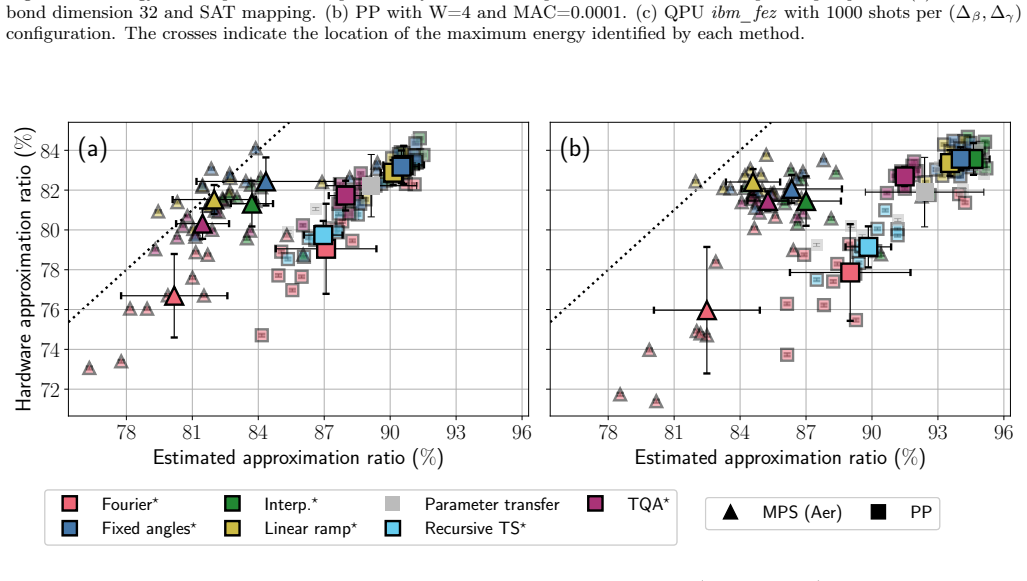
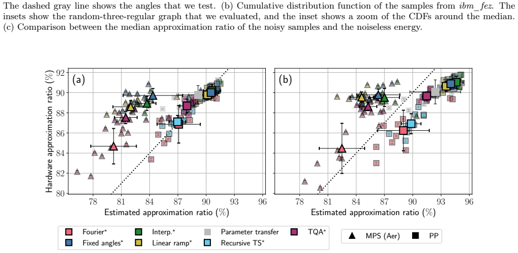
Line-based graphs Here, we repeat the analysis of Sec. VB2, but on ten 100-node line-based graphs. The edges are generated by an even and an odd SWAP layer applied to a line of 100 qubits. Each edge has a±1weight chosen with a50%probability. Following the same procedure as in Sec. VB2, we report the hardware approximation ratio against the training approx...
-
[16]
(FA, PP)⋆ – 1 2.1e-22.5e-21.6e-41.1e-135.2e-154.5e-214.0e-23 82.5 1 1 1 2.2e-1 2.3e-169.5e-122.8e-71.3e-16 75.9
-
[17]
(PT, PP) – – 2.1e-1 2.3e-13.4e-36.0e-122.8e-132.0e-191.6e-21 82.3 – 1 1 1 1.7e-147.6e-101.5e-58.7e-15 75.8
-
[18]
(I, PP)⋆ – – – 1 6.6e-1 1.3e-76.8e-93.7e-152.2e-17 81.7 – – 1 2.9e-1 5.7e-162.4e-116.2e-72.9e-16 75.9
-
[19]
(TQA, PP)⋆ – – – – 6.6e-1 9.4e-84.9e-92.6e-151.6e-17 81.7 – – – 2.0e-1 1.7e-167.2e-122.1e-79.2e-17 75.9
-
[20]
(F, PP)⋆ – – – – – 6.6e-54.5e-63.1e-121.8e-14 80.2 – – – – 9.0e-123.4e-72.6e-34.8e-12 74.5
-
[21]
(FA, MPSAer)⋆ – – – – – – 1 2.2e-33.5e-5 71.9 – – – – – 2.2e-1 1.4e-4 1 64.1
-
[22]
(I, MPSAer)⋆ – – – – – – – 1.8e-24.2e-4 71.6 – – – – – – 2.2e-1 1.7e-1 68.6
-
[23]
(TQA, MPSAer)⋆ – – – – – – – – 9.9e-1 68.7 – – – – – – – 8.3e-5 71.2
-
[24]
(F, MPSAer)⋆ – – – – – – – – – 68.2 – – – – – – – – 66.1 Methods(p=6) 1. 2. 3. 4. 5. 6. 7. 8. 9. Median 2. 3. 4. 5. 6. 7. 8. 9. Median
-
[25]
(PT, PP) – 6.7e-12.7e-31.3e-63.0e-129.3e-141.2e-124.6e-231.4e-24 93 2.4e-29.0e-17 1 1 1.2e-54.2e-182.3e-112.9e-16 76.8
-
[26]
(FA, PP)⋆ – – 1.6e-13.5e-42.4e-97.5e-119.7e-102.2e-205.5e-22 91.9 – 1.1e-102.9e-34.7e-3 2.2e-14.3e-121.5e-53.7e-10 75.6
-
[27]
(I, MPSAer)⋆ – – – 2.3e-1 3.2e-51.6e-61.4e-54.9e-169.8e-18 91.3 – – 4.2e-188.3e-181.5e-6 1 5.7e-2 1 64.7
-
[28]
(I, PP)⋆ – – – – 3.0e-23.1e-31.8e-25.7e-121.1e-13 89.7 – – – 1 7.3e-71.9e-199.3e-131.3e-17 77
-
[29]
(TQA, PP)⋆ – – – – – 1 1 2.1e-65.9e-8 88.1 – – – – 1.4e-63.8e-191.9e-122.6e-17 77
-
[30]
(F, PP)⋆ – – – – – – 1 4.1e-51.5e-6 87.6 – – – – – 7.2e-82.7e-24.3e-6 73.5
-
[31]
(FA, MPSAer)⋆ – – – – – – – 4.9e-61.4e-7 87.5 – – – – – – 8.1e-3 1 63.2
-
[32]
(TQA, MPSAer)⋆ – – – – – – – – 1 72.3 – – – – – – – 1.1e-1 71.2
-
[33]
(F, MPSAer)⋆ – – – – – – – – – 69.2 – – – – – – – – 66 Table VIII. Conover–Iman post-hoc test with Holm correction on estimated (left) and hardware (right) ratios generated from 10 100-node line-based graphs with 2 swap layers atp= 2(top) andp= 6(bottom). indicates p-values less than 0.05, indicates p-values less than 0.01, and indicates p-values less tha...
-
[34]
Abbas, A
A. Abbas, A. Ambainis, B. Augustino, A. Bärtschi, H. Buhrman, C. Coffrin, G. Cortiana, V. Dunjko, D. J. Egger, B. G. Elmegreen,et al., Challenges and oppor- tunities in quantum optimization, Nat. Rev. Phys.6, 718–735 (2024)
2024
-
[35]
E. Farhi, J. Goldstone, and S. Gutmann, A quan- tum approximate optimization algorithm (2014), arXiv:1411.4028
Pith/arXiv arXiv 2014
-
[36]
Wurtz and P
J. Wurtz and P. Love, MaxCut quantum approximate optimization algorithm performance guarantees forp > 1, Phys. Rev. A103, 042612 (2021)
2021
-
[37]
Bittel and M
L. Bittel and M. Kliesch, Training variational quantum algorithms is NP-hard, Phys. Rev. Lett.127, 120502 (2021)
2021
-
[38]
V. Vijendran, D. E. Koh, E. Bae, H. Kwon, P. K. Lam, and S. M. Assad, Near-optimal parameter tuning of level-1 qaoa for ising models (2025), arXiv:2501.16419
arXiv 2025
-
[39]
M. X. Goemans and D. P. Williamson, Improved ap- proximation algorithms for maximum cut and satisfia- bility problems using semidefinite programming, Jour- nal of the ACM (JACM)42, 1115 (1995)
1995
-
[40]
Khot, On the unique games conjecture (invited sur- vey), in2010 IEEE 25th annual conference on compu- tational complexity(IEEE Computer Society, 2010) pp
S. Khot, On the unique games conjecture (invited sur- vey), in2010 IEEE 25th annual conference on compu- tational complexity(IEEE Computer Society, 2010) pp. 99–121
2010
- [41]
-
[42]
Mastropietro, G
D. Mastropietro, G. Korpas, V. Kungurtsev, and J. Marecek, Parallel variational quantum algorithms with gradient-informed restart to speed up optimization in the presence of barren plateaus, IEEE Transactions on Quantum Engineering7, 1 (2026)
2026
-
[43]
Kungurtsev, G
V. Kungurtsev, G. Korpas, J. Marecek, and E. Y. Zhu, Iteration Complexity of Variational Quantum Al- gorithms, Quantum8, 1495 (2024)
2024
-
[44]
Bittel, S
L. Bittel, S. Gharibian, and M. Kliesch, The optimal depth of variational quantum algorithms is QCMA- hard to approximate, in38th Computational Complexity Conference (CCC 2023), Leibniz International Proceed- ings in Informatics (LIPIcs), Vol. 264 (Schloss Dagstuhl – Leibniz-Zentrum für Informatik, 2023) pp. 34:1–34:24
2023
- [45]
-
[46]
Bravyi, A
S. Bravyi, A. Kliesch, R. Koenig, and E. Tang, Obsta- cles to variational quantum optimization from symme- try protection, Phys. Rev. Lett.125, 260505 (2020)
2020
-
[47]
Bravyi, A
S. Bravyi, A. Kliesch, R. Koenig, and E. Tang, Hybrid quantum-classical algorithms for approximate graph coloring, Quantum6, 678 (2022)
2022
-
[48]
Hatami, L
H. Hatami, L. Lovász, and B. Szegedy, Limits of locally– globally convergent graph sequences, Geom. Funct. Anal.24, 269 (2014)
2014
-
[49]
Barak and K
B. Barak and K. Marwaha, Classical algorithms and quantum limitations for maximum cut on high-girth graphs, in13th Innovations in Theoretical Computer Science Conference (ITCS 2022), LIPIcs, Vol. 215 (Schloss Dagstuhl – Leibniz-Zentrum für Informatik,
2022
-
[50]
C.-N. Chou, P. J. Love, J. S. Sandhu, and J. Shi, Limitations of Local Quantum Algorithms on Random MAX-k-XOR and Beyond, in49th International Col- loquium on Automata, Languages, and Programming (ICALP 2022), Leibniz International Proceedings in In- formatics (LIPIcs), Vol. 229, edited by M. Bojańczyk, E. Merelli, and D. P. Woodruff (Schloss Dagstuhl – L...
2022
-
[51]
Mézard, T
M. Mézard, T. Mora, and R. Zecchina, Clustering of so- lutions in the random satisfiability problem, Phys. Rev. Lett.94, 197205 (2005)
2005
-
[52]
Achlioptas, A
D. Achlioptas, A. Coja-Oghlan, and F. Ricci-Tersenghi, On the solution-space geometry of random constraint satisfactionproblems,RandomStructures&Algorithms 38, 251 (2011)
2011
-
[53]
Gamarnik and M
D. Gamarnik and M. Sudan, Limits of local algorithms over sparse random graphs, inProceedings of the 5th Conference on Innovations in Theoretical Computer Science, ITCS ’14 (Association for Computing Machin- ery, New York, NY, USA, 2014) p. 369–376
2014
-
[54]
W.-K. Chen, D. Gamarnik, D. Panchenko, and M. Rah- man, Suboptimality of local algorithms for a class of max-cut problems, Anna. Probab.47, 1587 (2019)
2019
-
[55]
Gamarnik, The overlap gap property: A topologi- cal barrier to optimizing over random structures, Proc
D. Gamarnik, The overlap gap property: A topologi- cal barrier to optimizing over random structures, Proc. Natl. Acad. Sci.118, e2108492118 (2021)
2021
-
[56]
A. Chen, N. Huang, and K. Marwaha, Local algorithms and the failure of log-depth quantum advantage on sparse random CSPs (2023), arXiv:2310.01563
arXiv 2023
-
[57]
D. J. Egger, J. Mareček, and S. Woerner,Warm-starting quantum optimization, Quantum5, 479 (2021)
2021
-
[58]
R. Tate, J. Moondra, B. Gard, G. Mohler, and S. Gupta, Warm-started QAOA with custom mix- ers provably converges and computationally beats Goemans-Williamson’s max-cut at low circuit depths, Quantum7, 1121 (2023)
2023
-
[59]
Truger, J
F. Truger, J. Barzen, M. Bechtold, M. Beisel, F. Ley- mann, A. Mandl, and V. Yussupov, Warm-starting and quantum computing: A systematic mapping study, ACM Comput. Surv.56, 1 (2024)
2024
-
[60]
Tate and S
R. Tate and S. Eidenbenz, Warm-started QAOA with aligned mixers converges slowly near the poles of the Bloch sphere, inInternational Conference on Current Trends in Theory and Practice of Computer Science (Springer, 2025) pp. 311–323
2025
-
[61]
Schollwöck, The density-matrix renormalization group in the age of matrix product states, Ann
U. Schollwöck, The density-matrix renormalization group in the age of matrix product states, Ann. Phys. 326, 96–192 (2011)
2011
-
[62]
Y.Zhou, E.M.Stoudenmire,andX.Waintal,Whatlim- its the simulation of quantum computers?, Phys. Rev. X10, 041038 (2020)
2020
-
[63]
M. S. Rudolph, T. Jones, Y. Teng, A. Angrisani, and Z. Holmes, Pauli propagation: A computational framework for simulating quantum systems (2025), arXiv:2505.21606
Pith/arXiv arXiv 2025
-
[64]
P. Rall, D. Liang, J. Cook, and W. Kretschmer, Simu- lation of qubit quantum circuits via pauli propagation, Phys. Rev. A99, 062337 (2019)
2019
-
[65]
Willsch, M
D. Willsch, M. Willsch, F. Jin, K. Michielsen, and H. De Raedt, GPU-accelerated simulations of quan- 36 tum annealing and the quantum approximate optimiza- tion algorithm, Comput. Phys. Commun.278, 108411 (2022)
2022
-
[66]
S. H. Sack and M. Serbyn, Quantum annealing initial- ization of the quantum approximate optimization algo- rithm, Quantum5, 491 (2021)
2021
-
[67]
J. A. Montañez-Barrera and K. Michielsen, Toward a linear-ramp QAOA protocol: evidence of a scaling advantage in solving some combinatorial optimization problems, npj Quantum Inf.11, 131 (2025)
2025
-
[68]
K.McDowall, K.Georgopoulos,andP.Wallden,Aspec- tral gap informed parameter schedule for QAOA (2026), arXiv:2604.24580
Pith/arXiv arXiv 2026
-
[69]
S. Boulebnane, J. Sud, R. Shaydulin, and M. Pis- toia, Equivalence of Quantum Approximate Opti- mization Algorithm and Linear-Time Quantum An- nealing for the Sherrington-Kirkpatrick model (2025), arXiv:2503.09563
arXiv 2025
-
[70]
Wurtz and P
J. Wurtz and P. J. Love, Counterdiabaticity and the quantum approximate optimization algorithm, Quan- tum6, 635 (2022)
2022
-
[71]
A. B. Magann, K. M. Rudinger, M. D. Grace, and M. Sarovar, Feedback-based quantum optimization, Phys. Rev. Lett.129, 250502 (2022)
2022
-
[72]
V.Akshay, D.Rabinovich, E.Campos,andJ.Biamonte, Parameter concentrations in quantum approximate op- timization, Phys. Rev. A104, L010401 (2021)
2021
-
[73]
F. G. S. L. Brandao, M. Broughton, E. Farhi, S. Gut- mann, and H. Neven, For fixed control parameters the quantum approximate optimization algorithm’s objec- tive function value concentrates for typical instances (2018), arXiv:1812.04170
Pith/arXiv arXiv 2018
-
[74]
Shaydulin, I
R. Shaydulin, I. Safro, and J. Larson, Multistart Meth- ods for Quantum Approximate optimization, in2019 IEEE High Performance Extreme Computing Confer- ence (HPEC)(2019) pp. 1–8
2019
-
[75]
Galda, X
A. Galda, X. Liu, D. Lykov, Y. Alexeev, and I. Safro, Transferabilityofoptimalqaoaparametersbetweenran- dom graphs, in2021 IEEE International Conference on Quantum Computing and Engineering (QCE)(2021) pp. 171–180
2021
-
[76]
J. A. Montañez-Barrera, D. Willsch, and K. Michielsen, Transfer learning of optimal QAOA parameters in com- binatorial optimization, Quantum Inf. Process.24, 129 (2025)
2025
-
[77]
Pelofske, M
E. Pelofske, M. M. Rams, A. Bärtschi, P. Czarnik, P. Braccia, L. Cincio, and S. Eidenbenz, Evaluating the limits of Quantum Approximate Optimization Algo- rithm parameter transfer at high rounds on sparse Ising models with geometrically local cubic terms, Phys. Rev. Res.8, 023023 (2026)
2026
-
[78]
Pelofske, A
E. Pelofske, A. Bärtschi, L. Cincio, J. Golden, and S. Ei- denbenz, Scaling whole-chip QAOA for higher-order ising spin glass models on heavy-hex graphs, npj Quan- tum Inf.10, 109 (2024)
2024
-
[79]
S. V. Barron, D. J. Egger, E. Pelofske, A. Bärtschi, S. Eidenbenz, M. Lehmkuehler, and S. Woerner, Prov- able bounds for noise-free expectation values computed from noisy samples, Nat. Comput. Sci.4, 865–875 (2024)
2024
-
[80]
Kotil, E
A. Kotil, E. Pelofske, S. Riedmüller, D. J. Egger, S. Ei- denbenz, T. Koch, and S. Woerner, Quantum approx- imate multi-objective optimization, Nat. Comput. Sci. 5, 1168–1177 (2025)
2025
discussion (0)
Sign in with ORCID, Apple, or X to comment. Anyone can read and Pith papers without signing in.