REVIEW 2 major objections 6 minor 6 references
Community Detection on a Randomly Growing Network
T0 review · 2 major / 6 minor · reviewed 2026-07-12 · grok-4.5
Pith's one-line read You cannot label every node correctly in a growing preferential-attachment network with noise, but you can perfectly recover the early hubs and cores that define the communities.
desk verdict Solid first rigorous local-recovery theory for planted preferential-attachment forests; impossibility plus SPAR are cleanly scoped and the proofs hold. read the letter →
The pith
A machine-rendered reading of the paper's core claim, the machinery that carries it, and where it could break.
The reading
What carries the argument
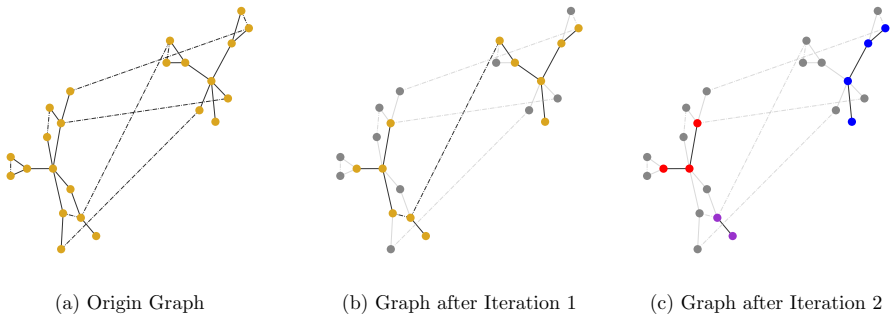
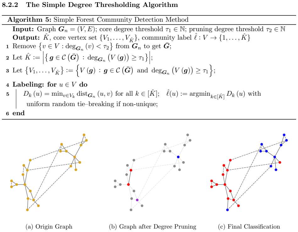
Selective Pruning with Anchor-based Recovery (SPAR): iterative removal of lowest-degree nodes that lie on cycles or whose deletion increases the number of high-degree components, isolating K anchor cores that seed distance- or posterior-based label propagation.
What would settle it
Generate planted forests with noise probability above the critical degree scale $n^{-(1+\alpha)/(2+\alpha)}$ and check whether SPAR still isolates the true community roots or whether high-degree nodes become randomly mixed across communities.
Extended reading notes
Core claim
Under the planted forest model with balanced community sizes and noise probability decaying slightly faster than the preferential-attachment degree scale, consistent recovery of every node is information-theoretically impossible, yet a simple pruning-plus-propagation algorithm recovers the labels of early-arriving, high-degree, and near-root nodes with zero or vanishing local misclustering error.
Load-bearing premise
The random noise edges must be sparse enough that the degrees of early nodes still track their arrival order; denser noise erases the signal that pruning relies on.
Editorial analysis
A structured set of objections, weighed in public.
Referee Report
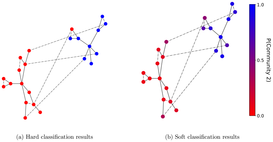
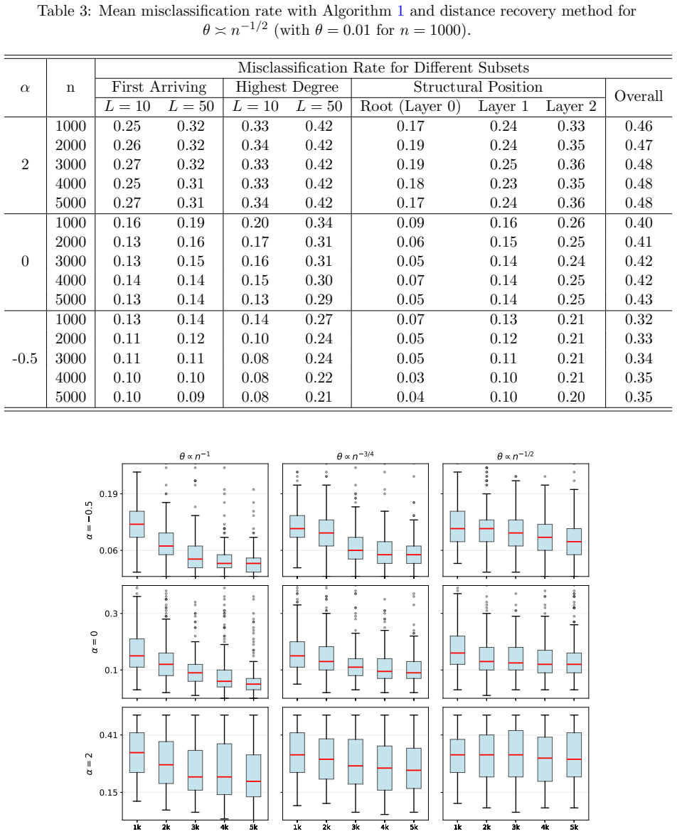
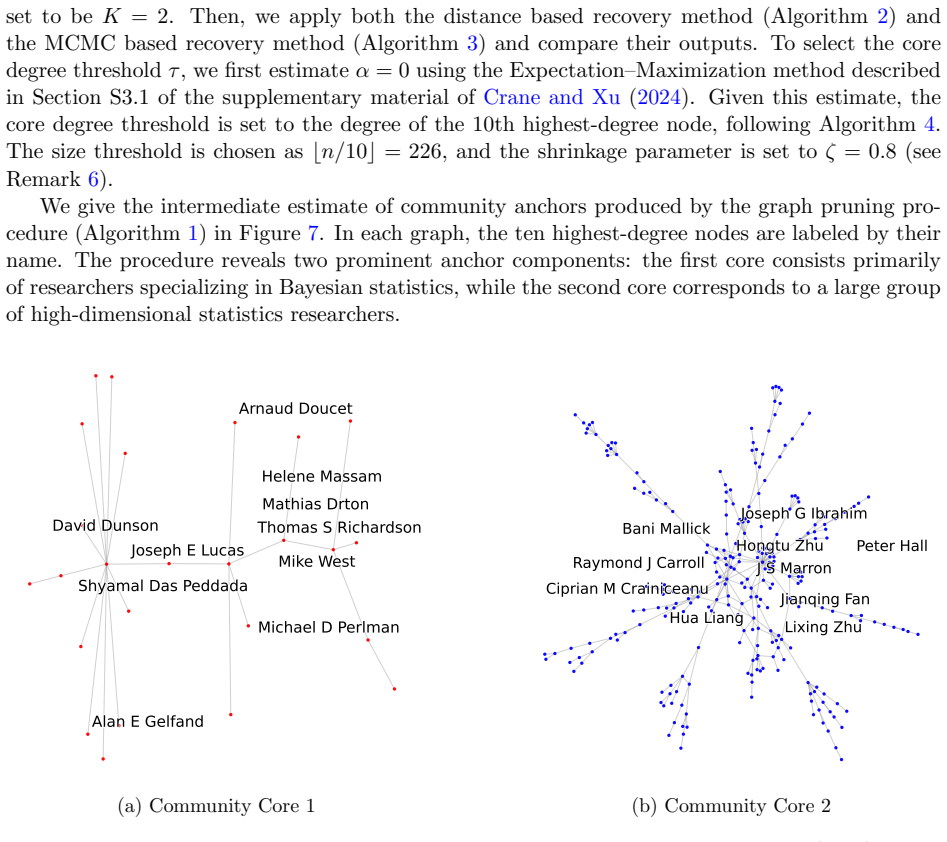
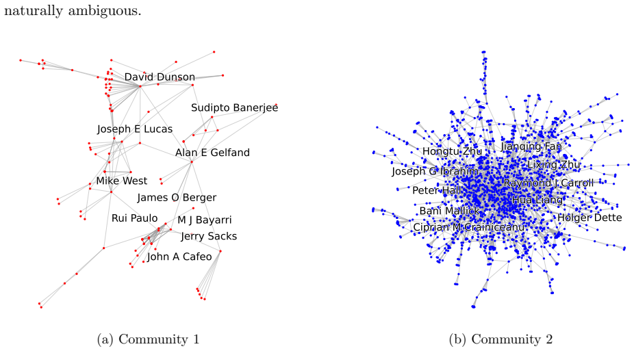
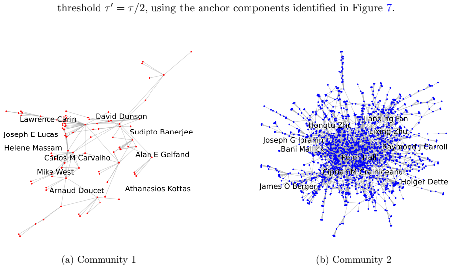
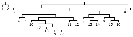
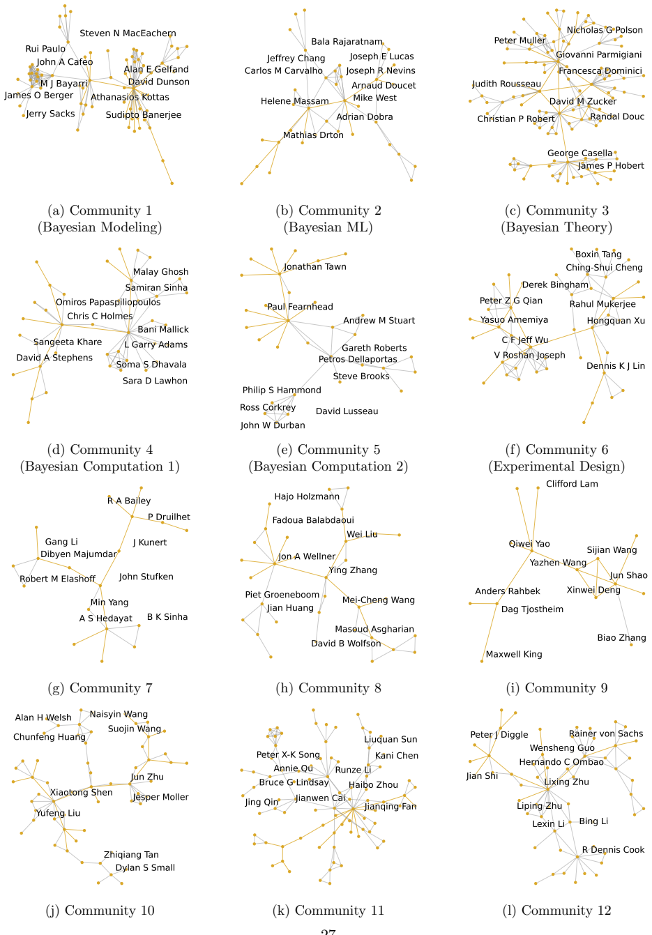
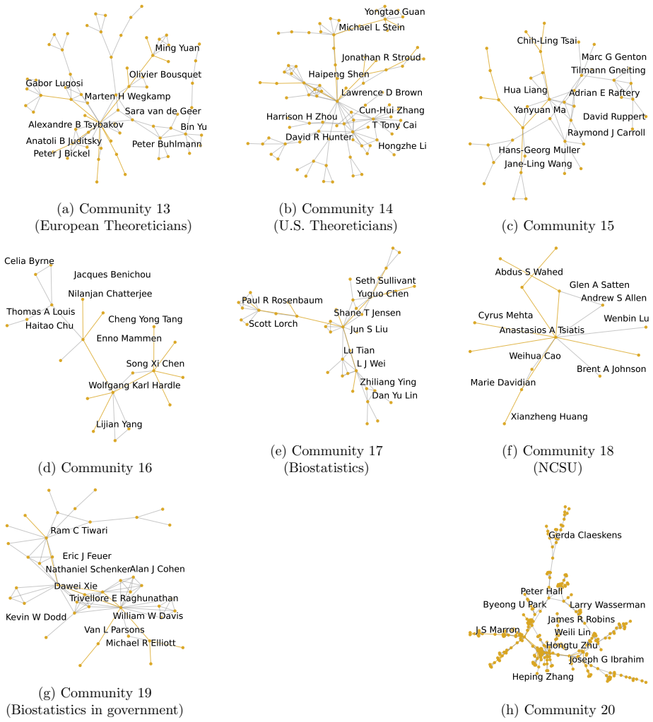
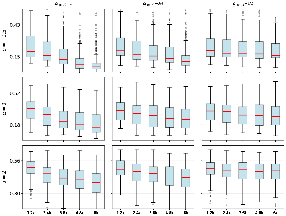
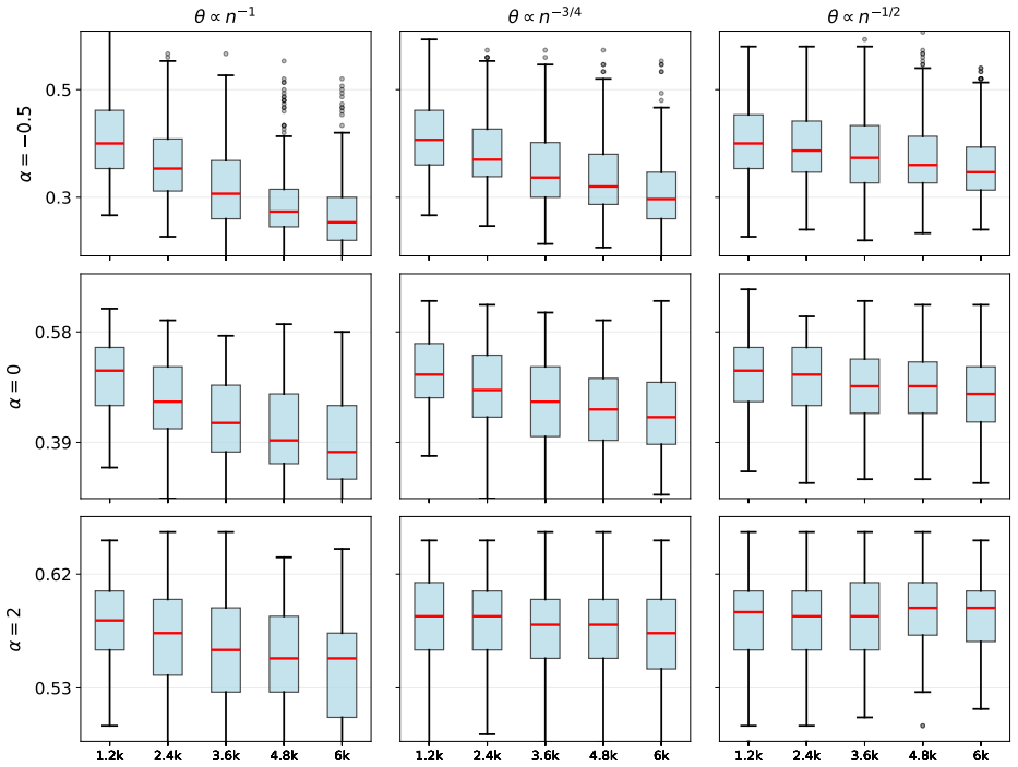
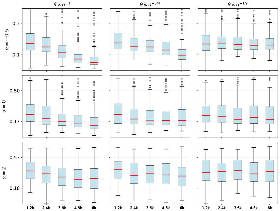
Summary. The paper studies community detection outside the SBM, under a planted forest model in which K independent affine preferential-attachment trees are superposed with Erdős–Rényi noise. It proves that no estimator can drive the global misclustering rate to zero when θ ≥ c/n (Theorem 1), then proposes SPAR: iterative degree-based pruning to extract K high-degree anchor components, followed by distance- or model-based label propagation. Under balanced community sizes and θ ≤ C0 n^{-(1+α)/(2+α)-δ}, SPAR recovers the first L arrivals of each community with zero local error w.h.p. (Theorem 2), recovers high-degree nodes perfectly (Corollary 1), and achieves vanishing local error on layer-1 nodes and, when α=0, layer-2 nodes (Theorem 3). Simulations across α and noise rates, plus a hierarchical analysis of the Ji–Jin coauthorship network, support the theory; code is public.
Significance. The work fills a genuine gap: community detection with rigorous guarantees for networks formed by sequential growth rather than independent edges. The impossibility result cleanly motivates local recovery, and the local guarantees (early arrivals, high degree, layers 1–2) are non-trivial and matched to preferential-attachment degree asymptotics. SPAR is simple, computationally efficient (O(|V|·|E|·deg(G))), and only loosely tied to the tree assumption, which is a methodological strength. Public code and a coherent real-data hierarchical clustering further raise the contribution. Limitations (known K, layer-2 only for α=0, noise-rate restriction) are scoped honestly and do not undercut the central claims as stated.
major comments (2)
- [Section 4, Remarks 4 and 10] Section 4 / Remark 4 and Remark 10: The main theorems treat K as known. Algorithm 5 gives a consistent estimator under the planted forest model, but the authors correctly note that τ2 is hard to tune in practice and that they fall back to hierarchical K=2 on real data. For a methods paper this is load-bearing for applicability: either strengthen the practical guidance for Algorithm 5 (or an alternative) with simulation evidence under misspecification, or state more clearly that hierarchical bipartition is the recommended operational procedure and report sensitivity of the coauthorship hierarchy to the leaf-size cutoff (currently 10).
- [Theorem 3, Remark 12, Section 2.4] Theorem 3 and Remark 12: Layer-2 recovery is proved only for α=0, and s≥3 is left open because misclassification accumulates across layers. The conjecture |Ls| ≍ n^{1/(2+α)} log^{s-1} n is plausible but unproved. This does not invalidate the stated theorems, but the abstract and introduction advertise recovery for “subsets of central nodes” including structural layers; a short, explicit statement of the α=0 restriction for layer 2 (and the barrier for s≥3) in the main-text overview (Section 2.4) would prevent over-reading of the guarantees.
minor comments (6)
- [Assumption 2, Table 4] Assumption 2: The noise threshold n^{-(1+α)/(2+α)} is well motivated by degree scales, and simulations (Table 4) suggest δ may be zero at the critical rate. A one-sentence conjecture in Section 4 or 7 would be useful for follow-up work.
- [Section 3.1, Algorithm 1] Algorithm 1: Degree is always computed w.r.t. the original Gn (not updated). This is justified for analysis (Remark after Algorithm 1); a brief note on whether updating degrees changes empirical performance would help practitioners.
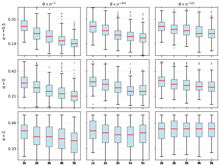
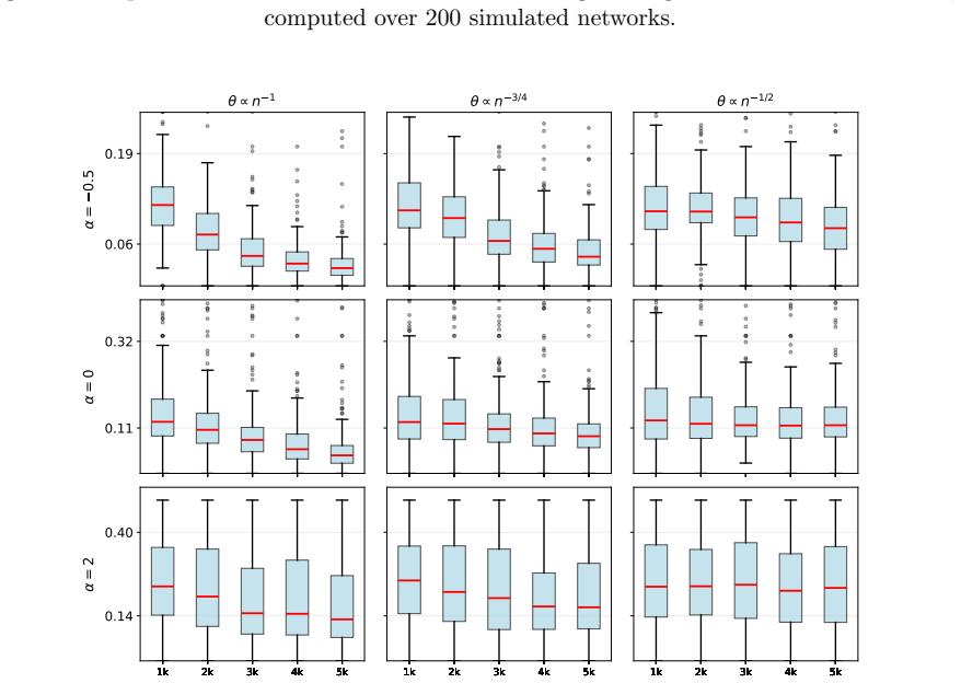
- [Section 5, Figures 4–6] Figures 4–6 and S2–S4: Boxplots are informative but dense; ensuring consistent y-axis scales within each α panel (or adding a short caption note) would improve readability.
- [Definition 2, Theorem 2] Notation: The dual use of π for global and community-specific orderings (Definition 2) is clear once stated, but a single reminder when π1:L(T^i) first appears in Theorem 2 would help.
- [Section 1.1] Related work: The distinction from Ben-Hamou–Velona and Hajek–Sankagiri (class-dependent attachment vs. disjoint growth; known vs. unknown arrival times) is well drawn; a sentence on how SPAR relates to leaf-stripping root-finding (Addario-Berry et al. 2025) beyond the brief mention would complete the picture.
- [Throughout] Typos / polish: “affine” / “Erdös” spelling is inconsistent in places (e.g., “Erdös–Rényi” vs “Erdős–Rényi”); “difficult” appears with ligature issues in the PDF source. Standardize.
Circularity Check
No significant circularity: local recovery guarantees are derived from the planted-forest generative assumptions plus external preferential-attachment degree asymptotics, not by construction from fitted targets or load-bearing self-citation.
full rationale
The central claims (global impossibility under θ=Ω(1/n); zero/vanishing local misclustering on early-arriving, high-degree and layer-1/2 nodes under the stated noise and balance assumptions) are proved from first principles inside the paper. Theorem 1 uses an information-theoretic indistinguishability argument via balanced-attachment events At (Appendix S1). Theorems 2–3 and Corollary 1 reduce the SPAR pruning-plus-distance procedure to known almost-sure degree-order limits for affine preferential attachment (Sénizergues 2021; Rudas et al. 2007; Lemmas 5–7, 14–17) together with elementary noise-control arguments under Assumption 2; the proofs never redefine the target error rates in terms of the algorithm outputs. Self-citations to Crane & Xu (2021, 2024) supply only the model name, the EM estimator for α, and the Gibbs sampler used in the optional model-based recovery stage; they are not invoked to justify uniqueness, to smuggle an ansatz, or to force the recovery rates. Free tuning parameters (τ, Q, τ′) appear in the algorithm statement and in simulations but are not used to define or fit the asymptotic error bounds. Consequently the derivation chain is self-contained against external benchmarks and exhibits only ordinary, non-load-bearing self-citation.
Assumptions & free parameters
free parameters (4)
- anchor-degree threshold τ (and recovery threshold τ′)
- anchor-size threshold Q (and shrinkage ζ)
- attachment parameter α and noise θ
- community count K
assumptions (6)
- domain assumption Communities are generated as independent affine preferential-attachment trees (Definition 1–2), with labels inherited from the tree of attachment.
- domain assumption Between-community edges are i.i.d. Erdős–Rényi with probability θ (Definition 2).
- domain assumption Assumption 1: each community size nk ≥ n/H for fixed H ≥ K (balanced communities).
- domain assumption Assumption 2: θ ≤ C0 n^{-(1+α)/(2+α)-δ} for some δ>0.
- standard math APA degree asymptotics: n^{-1/(2+α)} degrees of ordered nodes converge to a random sequence (Yj,α) in ℓq (Sénizergues; Lemmas 14–17).
- standard math For α=0, E|Ls(Tn)| ≍ √n (log n)^{s-1} (Lemma 11).
invented entities (3)
-
Planted forest model PF(α,θ,ℓ,π) / RC-PF
-
SPAR (Selective Pruning with Anchor-based Recovery)
independent evidence
-
Anchor components / high-degree cores after pruning
Cite this review
Pith. "Pith review of Community Detection on a Randomly Growing Network." pith.science (2026). https://pith.science/paper/VAMHOTK4
@misc{pith2026260607447,
  author       = {Pith},
  title        = {Pith review of: Community Detection on a Randomly Growing Network},
  year         = {2026},
  howpublished = {\url{https://pith.science/paper/VAMHOTK4}},
  note         = {Machine review of arXiv:2606.07447}
}
abstract
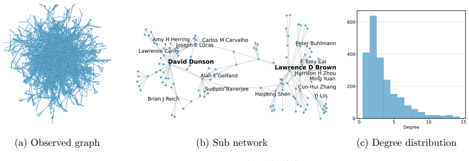
We study community detection on Markovian random networks outside of the Stochastic Block Model (SBM) framework. Specifically, we consider a random network growth process which generates $K$ separate preferential attachment trees and connects them with Erd\H{o}s--R\'enyi edges, so that each tree represents a community and each node inherits the label of the tree to which it belongs. This model is able to produce many features of real world networks that are improbable under SBM, such as power law degree distribution and the existence of chains and hubs. Given only the final graph, without any knowledge of the growth process, we seek to recover the unobserved community membership of the nodes. We first prove that it is impossible for any algorithm to consistently recover the community label of all the nodes. However, we design algorithms which are provably able to recover the community labels of subsets of central nodes, for several different notions of node centrality such as arrival time or degree. Our procedure consists of two stages where, in the first stage, we classify high degree nodes and then, in the second stage, extend the community assignments to the remaining vertices. Numerical experiments and a real data application on a coauthorship network demonstrate the effectiveness of our proposed approach.
Figures

Figures from the paper (27 more)













Reference graph
Works this paper leans on
-
[1]
A. Cerqueira and E. Levina. A pseudo-likelihood approach to community detection in weighted networks. arXiv preprint arXiv:2303.05909 ,
-
[2]
C. Xin, F. Xu, X. Ding, J. Gao, and J. Ding. Toping: Topologically interpretable graph learning via persistent rationale filtration. arXiv preprint arXiv:2510.05102 ,
-
[3]
E. Yanchenko, S. Sengupta, and D. Mukherjee. Statistical inference for core-periphery structures. arXiv preprint arXiv:2508.04730 ,
-
[4]
If the graph parameters (α, θ) are assumed to be unknown, the noise level θ can still be easy to estimate, e.g
Algorithm 4 assumes the graph parameters (α, θ) are available. If the graph parameters (α, θ) are assumed to be unknown, the noise level θ can still be easy to estimate, e.g. by ˆθ = |E(Gn)|−n+1 |E(Gn)| . By contrast, α can be harder to estimate. A principled estimation procedure is given in the supplementary material of Crane and Xu (2024). In practice, ...
2024
-
[5]
This completes the proof of ( S4.41)
ε. This completes the proof of ( S4.41). S4.5 Technical Lemmas Lemma 13 (Theorem 2 in Rudas et al. (2007)). For Tn APA(α, n) with α >1, as n!1 , v : degTn (v) = 1 n P!p (1) > 0, that is, the proportion of degree- 1 vertices converges in probability to a positive constant p(1) that depends on α. Lemma 14 (Proposition 5.5 in Sénizergues (2021)). Let q > 2 +...
2007
-
[6]
Let X be a random variable with Bin(n, θ) distribution
65 Lemma 18 (Lemma S8 in Crane and Xu (2024)). Let X be a random variable with Bin(n, θ) distribution. For any q 1, θ2 [0, 1] and any n2 N, we have that EX q (2θn)q + Cq, where Cq > 0 is a constant that depends only on q. Proof. Write X as a random variable with the Bin(n, θ) distribution. Then, EX q = Z ∞ 0 P (X q t) dt (2θn)q + Z ∞ (2θn)q P (X q t) dt (...
2024
Reviewed July 12, 2026 · model on record in the stance chip above.
Discussion (0). Continue with ORCID to comment.