pith. sign in

arxiv: 2606.08316 · v1 · pith:THPG2L63new · submitted 2026-06-06 · ✦ hep-lat

Some Inverse Problems in Particle Physics

Pith reviewed 2026-06-27 18:36 UTC · model grok-4.3

classification ✦ hep-lat
keywords inverse problemsparton distribution functionsspectral functionslattice QCDBackus-GilbertGaussian processesneural networks
0
0 comments X

The pith

Inverse problems central to particle phenomenology are solved using Backus-Gilbert, Gaussian Processes, and neural network methods for PDFs and spectral functions.

A machine-rendered reading of the paper's core claim, the machinery that carries it, and where it could break.

The paper aims to show that inverse problems are key in current particle physics research by focusing on extracting parton distribution functions from experimental or lattice data and spectral functions from lattice correlators. It examines three specific methods in detail to provide practical tools for these extractions. A reader would care because these extractions reveal fundamental properties of particles that cannot be measured directly. The work connects experimental data analysis with lattice QCD computations.

Core claim

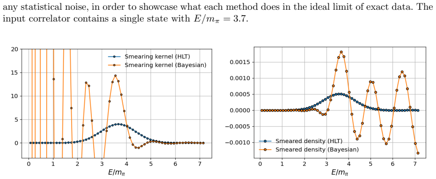
Inverse problems play a central role in particle phenomenology, and the three approaches of Backus-Gilbert, Gaussian Processes and neural network parametrizations can be used to extract Parton Distribution Functions from data or lattice pseudo- and quasi-PDFs, and spectral functions from Euclidean time correlators.

What carries the argument

Backus-Gilbert method, Gaussian Processes, and neural network parametrizations for solving inverse problems in PDF and spectral function extraction.

Load-bearing premise

That the three named methods are the main relevant approaches and can be meaningfully compared without further data on their performance limitations.

What would settle it

A benchmark study on identical lattice ensembles revealing significant differences in accuracy or bias among the three methods would test the investigation's value.

Figures

Figures reproduced from arXiv: 2606.08316 by Luigi Del Debbio.

Figure 1
Figure 1. Figure 1 [PITH_FULL_IMAGE:figures/full_fig_p026_1.png] view at source ↗
Figure 2
Figure 2. Figure 2: Samples from the posterior distribution of T3, plotted in linear (left panel) and log (right panel) scale. The dark blue line represent the mean of the distribution, while the black dotted line the input PDF, f0, used to generate pseudo-data. The shaded regions represent the 68CL and 95CL intervals, and in light blue we plot a few representative samples from the distribution. The posterior displays a small… view at source ↗
Figure 3
Figure 3. Figure 3: GP reconstruction of the input function f0, with the 68% CL band for the experimental and recon￾struction errors plotted separately in grey and red respectively, according to Eq. (126). The error bands are overlapped rather than stacked. Plot taken from Ref. [10]. 4.5.1 GP Solution and Connection with BG Following the formalism introduced in this section, we represent the spectral density as a stochastic f… view at source ↗
Figure 4
Figure 4. Figure 4: Combination of the stability analysis used (left) and a scan of the NLL (right). The smeared density shown in the left panel is obtained at a specific energy, and is evaluated from GPs, i.e. from Eqs. (143) and (144) for the central value and the error respectively. The prior is the modified Gaussian of Eq. (147), with ϵ ≃ m0, the latter being the ground state of the channel. We only display value correspo… view at source ↗
Figure 5
Figure 5. Figure 5: Left panel: examples of the function smearing the spectral density at the energy E = 3.7mπ in the Bayesian setup (orange) and from the HLT procedure (blue) using exact data. The latter targets a Gaussian kernel with a width of approximately 0.75 in units of mπ, which is reconstructed with great precision given the lack of uncertainties on the input data. For the Bayesian calculation, we use the same Gaussi… view at source ↗
Figure 6
Figure 6. Figure 6: A feed-forward neural network with L = 3 layers and n0 = 2, n1 = 25, n2 = 20, n3 = 8. The input layer is in green on the left, the output layer is in red on the right, and the hidden layers are in blue. This is the actual architecture of the neural network used by the NNPDF collaboration for PDF fitting, see Ref. [2]. 5.2 Neural Networks at Initialization The weights and biases of the NN are initialized as… view at source ↗
Figure 7
Figure 7. Figure 7: The empirical (left) and analytical (right) covariance matrices of the first, second and output layers of the NNPDF architecture (top to bottom). The covariance in the left panel is computed “bootstrapping” over an ensemble of replicas, initialized using the Glorot normal distribution. The covariance in the right panel is obtained by solving Eq. (176) numerically. In order to reduce the bootstrap errors in… view at source ↗
Figure 8
Figure 8. Figure 8: Relative difference between the empirical kernel, computed from an ensemble of networks at initializa￾tion, and the recursive kernel obtained by iterating Eq. (176) for the three layers of the NNPDF architecture. An ensemble of 1000 replicas has been used to reduce the bootstrap errors in the empirical covariance. −0.004 −0.002 0.000 0.002 0.004 f(x) 0 200 400 600 800 1000 p(f) [25, 20] Empirical Theory −0… view at source ↗
Figure 9
Figure 9. Figure 9: Sampled distribution of the output xT3 at x = 0.0065 for two different ensemble sizes, Nrep = 100 (top) and Nrep = 1000 (bottom). Each column shows the distribution for a different network architecture, the latter displayed in the top left corner of each panel. The red line the represents the predicted Gaussian distribution as dictated by the kernel recursion formula in Eq. (176). 42 [PITH_FULL_IMAGE:figu… view at source ↗
Figure 10
Figure 10. Figure 10: The output of the ensemble of neural networks at initialization using the NNPDF architecture in linear (left) and logarithm (right) scale. We compare the case of linear input f(x) (blue) and the case of scaled input f(x, log x) (orange). The solid lines represent the mean value computed over an ensemble of 100 replicas, while the shaded bands represent the one-sigma uncertainty computed as the variance ov… view at source ↗
Figure 11
Figure 11. Figure 11: Frobenius norm of the NTK at initialization, ∥Θ0∥, as a function of the width of the network. On the left, the central values and uncertainty bands are obtained as the mean and one-sigma deviation of the ensemble of networks. The labels on the horizontal axis indicate the respective widths of the two hidden layers in the networks considered.The plot on the right shows the relative uncertainty. It is inter… view at source ↗
Figure 12
Figure 12. Figure 12: Spectrum of the NTK at initialization for the architectures shown in [PITH_FULL_IMAGE:figures/full_fig_p048_12.png] view at source ↗
Figure 13
Figure 13. Figure 13: Relative variation of the NTK during training for L0, L1, and L2 data. Error bands correspond to one-sigma uncertainties over the ensemble of networks. for the three different datasets, L0, L1, and L2. Inspecting the plot reveals that the NTK undergoes significant changes during the initial phase of training, with the relative variation δΘt reaching values as high as 6%. This indicates that our settings d… view at source ↗
Figure 14
Figure 14. Figure 14: Evolution during training of the first five eigenvalues of the NTK using L0 (left), L1 (center), and L2 (right) data. Solid lines represent the median over the ensemble of networks, while solid bands correspond to 68% confidence level. Note that the subdominant eigenvalues λ (3) , λ (4) and λ (5) have increased by one or two orders of magnitude by the end of the rich training phase. In [PITH_FULL_IMAGE:f… view at source ↗
Figure 15
Figure 15. Figure 15: The first five eigenvalues of the NTK for L0, L1, and L2 data. Solid lines represent the median over the ensemble of networks, while solid bands correspond to 68% confidence level. Each plot corresponds to a different eigenvalue, as indicated by the label on the vertical axis. Note the different scales on the vertical axes, which reflects the hierarchy of eigenvalues discussed above. Different colours cor… view at source ↗
Figure 16
Figure 16. Figure 16: Variation of the loss function overlaid with the first five eigenvalues for a selected replica over the ensemble using L0 (left), L1 (center), and L2 (right) data. Left scale refers to the loss, while the right scale refers to the eigenvalues. 6.2.3 Eigenvectors as Features It has been argued above that there is a non-trivial interplay between the eigenspace of the NTK and that of the matrix M. Indeed, th… view at source ↗
Figure 17
Figure 17. Figure 17: Matrix A as defined in Eq. (193) for L2 data and for a single replica of the NTK. The matrix is shown at different epochs of the training process, indicated in the top of each panel. learnable directions – the features that the network can learn – are aligned with the directions that contribute most to the observables. 102 103 104 Epochs 0.0025 0.0050 0.0075 0.0100 0.0125 0.0150 0.0175 0.0200 Ct r = 4 r =… view at source ↗
Figure 18
Figure 18. Figure 18: Reconstruction error Ct(r) as defined in Eq. (194) as a function of the training time and for different numbers of eigenvectors r. Note that f0 lies entirely in the subspace spanned by the first four eigenvectors of the NTK by the onset of the lazy training regime. We see that the NTK has aligned its features with the physically relevant directions of the problem. The eigenvectors of the NTK form an ortho… view at source ↗
Figure 19
Figure 19. Figure 19: First five eigenvectors of the NTK at different training times and as function of the input x-grid. We also show the output of the network at the same training time, which is displayed in gray. L1 data is used. A complementary picture is displayed in [PITH_FULL_IMAGE:figures/full_fig_p053_19.png] view at source ↗
Figure 20
Figure 20. Figure 20: Evolution during training of the first five eigenvalues of H⊥ using L0 (left), L1 (center), and L2 (right) data. Solid lines represent the median over the ensemble of networks, while solid bands correspond to 68% confidence level. Note that the subdominant eigenvalues λ (3) , λ (4) and λ (5) have increased by one or two orders of magnitude by the end of the rich training phase. x −2 −1 0 1 2 3 q(x) T = 50… view at source ↗
Figure 21
Figure 21. Figure 21: First five eigenvectors of the combined matrix H = ΘM, as in Eq. (190), at different training times and as a function of the input x-grid. We also show the output of the network at the same training time, which is displayed in gray. L1 data is used. and 19), from which they are constructed. However, we see that h (i) are larger by around three orders of magnitude than the NTK eigenvalues. The solution to … view at source ↗
Figure 22
Figure 22. Figure 22: Comparison of the trained and analytical evolution at the end of training. Each panel corresponds to a different frozen NTK, whereby the analytical solution is computed starting from fTRef . The orange curve represents the final trained function after 50000 iterations of GD, and is the same across panels. Error bands represent one-sigma uncertainties across replicas. L2 data is used. A complementary persp… view at source ↗
Figure 23
Figure 23. Figure 23: Decomposition of the analytical solution into the two contributions from U and V at different training times. The frozen NTK is fixed across panels, and corresponds to the one at Tref = 10000. The initial condition for the analytical solution is always fTref . As in [PITH_FULL_IMAGE:figures/full_fig_p059_23.png] view at source ↗
Figure 24
Figure 24. Figure 24: Test of the t → ∞ limit of the L0 training for different frozen NTKs. The green curve represents the projection of the input function f0 onto the subspace orthogonal to the kernel of the NTK at tref, i.e., f ⊥ 0 . The purple curve represents the contribution of the operator V , computed with the NTK at Tref, in the limit of infinite training time. 0.0 0.2 0.4 0.6 0.8 1.0 x −0.0004 −0.0002 0.0000 0.0002 0.… view at source ↗
Figure 25
Figure 25. Figure 25: Test of the average of the parallel contribution for different epochs. The reference epoch at which the frozen NTK is chosen is Tref = 10000. L2 data is used in the plot. Note that the scale on the vertical axis is three orders of magnitude smaller than in [PITH_FULL_IMAGE:figures/full_fig_p061_25.png] view at source ↗
Figure 26
Figure 26. Figure 26: Comparison of the trained (orange) and analytical (blue) evolution starting from an ensemble of networks at initialization as the initial condition. Each row corresponds to a different frozen NTK, while the columns represent different training times. The dashed line represents the input function used to generate the synthetic data, i.e., the true result. L2 data is used. U(t) and f0. In the absence of suc… view at source ↗
Figure 27
Figure 27. Figure 27: Behaviour of ∆[U(t)f0] and ∆[V (t)Y ], as defined in Eqs. (240) and (241), as functions of the training time. The operators U(T) and V (T) are constructed by taking the NTK at Tref = 10000, which is fixed across panels. The uncertainties are extracted from the bootstrap ensemble as discussed in the text. Let us conclude this brief discussion by noting that Eq. (239) resembles the structure of a linear met… view at source ↗
Figure 28
Figure 28. Figure 28: Decomposition of the error budget of the trained fields into the two components from the initial condition (blue) and from the data (orange), as defined in Eqs. (234) and (236). Each row corresponds to a different frozen NTK, while the columns represent different training epochs. L2 data is used. We see that if the NTK is taken at later stages of training, the contribution from the initial condition is se… view at source ↗
Figure 29
Figure 29. Figure 29: Similar to [PITH_FULL_IMAGE:figures/full_fig_p068_29.png] view at source ↗
read the original abstract

Inverse problems play a central role in current areas of research in particle phenomenology. In these lectures we focus on two examples, the extraction of Parton Distribution Functions (PDFs) from experimental data (or, equivalently, from pseudo- and quasi-PDFs computed in lattice QCD), and the extraction of spectral functions from lattice Euclidean time correlators. We investigate in detail three different approaches, namely Backus-Gilbert, Gaussian Processes and fits based on Neural Network parametrizations.

Editorial analysis

A structured set of objections, weighed in public.

Desk editor's note, referee report, simulated authors' rebuttal, and a circularity audit. Tearing a paper down is the easy half of reading it; the pith above is the substance, this is the friction.

Referee Report

0 major / 1 minor

Summary. The manuscript consists of lecture notes reviewing inverse problems in particle phenomenology. It focuses on two standard examples—the extraction of parton distribution functions (PDFs) from experimental data or lattice QCD pseudo-/quasi-PDFs, and the extraction of spectral functions from Euclidean correlators—and examines three established methods in detail: the Backus-Gilbert approach, Gaussian processes, and neural-network parametrizations.

Significance. If the descriptions are accurate, the notes could serve as a pedagogical compilation of known techniques for lattice practitioners and phenomenologists. However, the text advances no new derivations, performance benchmarks, validation data, or falsifiable predictions, limiting its significance to exposition rather than original research.

minor comments (1)
  1. [Abstract] The abstract states that the three methods are 'investigated in detail,' yet the overall presentation remains at the level of known techniques without new quantitative comparisons or error analyses on specific lattice ensembles.

Simulated Author's Rebuttal

0 responses · 0 unresolved

We thank the referee for their positive assessment of the manuscript and the recommendation to accept. The work is explicitly presented as lecture notes reviewing established methods, with no claim to new derivations or benchmarks.

Circularity Check

0 steps flagged

No significant circularity; review of established methods

full rationale

The paper consists of lecture notes reviewing three established methods (Backus-Gilbert, Gaussian Processes, neural-network parametrizations) for two standard inverse problems in particle physics. No new derivations, predictions, or central claims are advanced that could reduce by construction to fitted inputs or self-citations. All content is expository of known techniques, with no load-bearing steps that equate outputs to inputs via definition or self-reference.

Axiom & Free-Parameter Ledger

0 free parameters · 0 axioms · 0 invented entities

As this is a review of known methods with no new central claim or derivation, no free parameters, axioms, or invented entities are introduced or relied upon beyond standard physics background.

pith-pipeline@v0.9.1-grok · 5586 in / 1052 out tokens · 37871 ms · 2026-06-27T18:36:47.573068+00:00 · methodology

discussion (0)

Sign in with ORCID, Apple, or X to comment. Anyone can read and Pith papers without signing in.

Reference graph

Works this paper leans on

29 extracted references · 17 canonical work pages · 3 internal anchors

  1. [1]

    Rothkopf, A.: Tackling inverse problems for PDFs from lattice QCD. (2026)

  2. [2]

    Ball, R.D.,et al.: The path to proton structure at 1% accuracy. Eur. Phys. J. C82(5), 428 (2022) https://doi.org/10.1140/epjc/s10052-022-10328-7 arXiv:2109.02653 [hep-ph]

  3. [3]

    Bailey, S., Cridge, T., Harland-Lang, L.A., Martin, A.D., Thorne, R.S.: Parton distributions from LHC, HERA, Tevatron and fixed target data: MSHT20 PDFs. Eur. Phys. J. C81(4), 341 (2021) https://doi.org/10.1140/epjc/s10052-021-09057-0 arXiv:2012.04684 [hep-ph]

  4. [4]

    Hou, T.-J.,et al.: New CTEQ global analysis of quantum chromodynamics with high-precision data from the LHC. Phys. Rev. D103(1), 014013 (2021) https://doi.org/10.1103/PhysRevD. 103.014013 arXiv:1912.10053 [hep-ph]

  5. [5]

    Salg, M., Romero-L´ opez, F., Jay, W.I.: Bayesian analysis and analytic continuation of scattering amplitudes from lattice QCD. Phys. Rev. D112(11), 114502 (2025) https://doi.org/10.1103/ ty19-xvvw arXiv:2506.16161 [hep-lat]

  6. [6]

    Mathematical Proceedings of the Cambridge Philosophical Society51(3), 406–413 (1955) https://doi.org/10.1017/S0305004100030401

    Penrose, R.: A generalized inverse for matrices. Mathematical Proceedings of the Cambridge Philosophical Society51(3), 406–413 (1955) https://doi.org/10.1017/S0305004100030401

  7. [7]

    1540-6261.1952.tb01525.x

    Backus, G.E., Gilbert, J.F.: Numerical applications of a formalism for geophysical inverse problems. Geophysical Journal International13(1-3), 247–276 (1967) https://doi.org/10.1111/j. 1365-246X.1967.tb02159.x https://academic.oup.com/gji/article-pdf/13/1-3/247/2722726/13-1- 3-247.pdf

  8. [9]

    Hansen, M., Lupo, A., Tantalo, N.: Extraction of spectral densities from lattice correlators. Phys. Rev. D99(9), 094508 (2019) https://doi.org/10.1103/PhysRevD.99.094508 arXiv:1903.06476 [hep-lat]

  9. [10]

    Candido, A., Del Debbio, L., Giani, T., Petrillo, G.: Bayesian inference with Gaussian processes for the determination of parton distribution functions. Eur. Phys. J. C84(7), 716 (2024) https: //doi.org/10.1140/epjc/s10052-024-13100-1 arXiv:2404.07573 [hep-ph]

  10. [11]

    Benvenuti, A.C.,et al.: A High Statistics Measurement of the Proton Structure Functions F(2) (x, Q**2) and R from Deep Inelastic Muon Scattering at High Q**2. Phys. Lett. B223, 485–489 (1989) https://doi.org/10.1016/0370-2693(89)91637-7

  11. [12]

    Del Debbio, L., Lupo, A., Panero, M., Tantalo, N.: Bayesian solution to the inverse problem and its relation to Backus–Gilbert methods. Eur. Phys. J. C85(2), 185 (2025) https://doi.org/10. 1140/epjc/s10052-025-13885-9 arXiv:2409.04413 [hep-lat] 71

  12. [13]

    Horak, J., Pawlowski, J.M., Rodr´ ıguez-Quintero, J., Turnwald, J., Urban, J.M., Wink, N., Zafeiropoulos, S.: Reconstructing QCD spectral functions with Gaussian processes. Phys. Rev. D 105(3), 036014 (2022) https://doi.org/10.1103/PhysRevD.105.036014 arXiv:2107.13464 [hep-ph]

  13. [14]

    A framework for probabilistic continuous inverse theory

    Valentine, A.P., Sambridge, M.: Gaussian process models—I. A framework for probabilistic continuous inverse theory. Geophysical Journal International220(3), 1632–1647 (2019) https://doi.org/10.1093/gji/ggz520 https://academic.oup.com/gji/article- pdf/220/3/1632/31578341/ggz520.pdf

  14. [15]

    JHEP07, 034 (2022) https: //doi.org/10.1007/JHEP07(2022)034 arXiv:2111.12774 [hep-lat]

    Bulava, J., Hansen, M.T., Hansen, M.W., Patella, A., Tantalo, N.: Inclusive rates from smeared spectral densities in the two-dimensional O(3) non-linearσ-model. JHEP07, 034 (2022) https: //doi.org/10.1007/JHEP07(2022)034 arXiv:2111.12774 [hep-lat]

  15. [16]

    Del Debbio, L., Lupo, A., Panero, M., Tantalo, N.: Multi-representation dynamics of SU(4) composite Higgs models: chiral limit and spectral reconstructions. Eur. Phys. J. C83(3), 220 (2023) https://doi.org/10.1140/epjc/s10052-023-11363-8 arXiv:2211.09581 [hep-lat]

  16. [17]

    Alexandrou, C.,et al.: Probing the Energy-Smeared R Ratio Using Lattice QCD. Phys. Rev. Lett.130(24), 241901 (2023) https://doi.org/10.1103/PhysRevLett.130.241901 arXiv:2212.08467 [hep-lat]

  17. [18]

    Bennett, E., et al.: Meson spectroscopy from spectral densities in lattice gauge theories (2024) arXiv:2405.01388 [hep-lat]

  18. [19]

    Geophysical Jour- nal International16(2), 169–205 (1968) https://doi.org/10.1111/j.1365-246X.1968.tb00216.x https://academic.oup.com/gji/article-pdf/16/2/169/5891044/16-2-169.pdf

    Backus, G., Gilbert, F.: The Resolving Power of Gross Earth Data. Geophysical Jour- nal International16(2), 169–205 (1968) https://doi.org/10.1111/j.1365-246X.1968.tb00216.x https://academic.oup.com/gji/article-pdf/16/2/169/5891044/16-2-169.pdf

  19. [20]

    In: Teh, Y.W., Titterington, M

    Glorot, X., Bengio, Y.: Understanding the difficulty of training deep feedforward neural networks. In: Teh, Y.W., Titterington, M. (eds.) Proceedings of the Thirteenth Interna- tional Conference on Artificial Intelligence and Statistics. Proceedings of Machine Learn- ing Research, vol. 9, pp. 249–256. PMLR, Chia Laguna Resort, Sardinia, Italy (2010). http...

  20. [21]

    Cambridge University Press, ??? (2022)

    Roberts, D.A., Yaida, S., Hanin, B.: The Principles of Deep Learning Theory: An Effective Theory Approach to Understanding Neural Networks. Cambridge University Press, ??? (2022). https://doi.org/10.1017/9781009023405 .http://dx.doi.org/10.1017/9781009023405

  21. [22]

    Chiefa, A., Del Debbio, L., Kenway, R.: Quantitative Understanding of PDF Fits and their Uncertainties (2025) arXiv:2512.24116 [hep-ph]

  22. [23]

    Barrett, D.G.T., Dherin, B.: Implicit gradient regularization (2022) arXiv:2009.11162 [cs.LG]

  23. [24]

    Advances in neural information processing systems31(2018) arXiv:1806.07572 [cs.LG] 72

    Jacot, A., Gabriel, F., Hongler, C.: Neural Tangent Kernel: Convergence and Generalization in Neural Networks. Advances in neural information processing systems31(2018) arXiv:1806.07572 [cs.LG] 72

  24. [25]

    Parton distributions for the LHC Run II

    Ball, R.D.,et al.: Parton distributions for the LHC Run II. JHEP04, 040 (2015) https://doi. org/10.1007/JHEP04(2015)040 arXiv:1410.8849 [hep-ph]

  25. [26]

    Journal of Sta- tistical Mechanics: Theory and Experiment2020(12), 124002 (2020) https://doi.org/10.1088/ 1742-5468/abc62b arXiv:1902.06720 [stat.ML]

    Lee, J., Xiao, L., Schoenholz, S., Bahri, Y., Novak, R., Sohl-Dickstein, J., Pennington, J.: Wide neural networks of any depth evolve as linear models under gradient descent. Journal of Sta- tistical Mechanics: Theory and Experiment2020(12), 124002 (2020) https://doi.org/10.1088/ 1742-5468/abc62b arXiv:1902.06720 [stat.ML]

  26. [27]

    Advances in Neural Information Processing Systems33, 5850–5861 (2020) arXiv:2010.15110 [cs.LG]

    Fort, S., Dziugaite, G.K., Paul, M., Kharaghani, S., Roy, D.M., Ganguli, S.: Deep learning versus kernel learning: an empirical study of loss landscape geometry and the time evolution of the neural tangent kernel. Advances in Neural Information Processing Systems33, 5850–5861 (2020) arXiv:2010.15110 [cs.LG]

  27. [28]

    Ablat, A.,et al.: New results in the CTEQ-TEA global analysis of parton distributions in the nucleon. Eur. Phys. J. Plus139(11), 1063 (2024) https://doi.org/10.1140/epjp/ s13360-024-05865-x arXiv:2406.10260 [hep-ph]

  28. [29]

    Alekhin, S., Bl¨ umlein, J., Moch, S., Placakyte, R.: Parton distribution functions,α s, and heavy- quark masses for LHC Run II. Phys. Rev. D96(1), 014011 (2017) https://doi.org/10.1103/ PhysRevD.96.014011 arXiv:1701.05838 [hep-ph]

  29. [30]

    Costantini, M.N., Mantani, L., Moore, J.M., Ubiali, M.: A linear PDF model for Bayesian inference (2025) arXiv:2507.16913 [hep-ph] Data Availability Statement: No new data were created or analysed in this study. 73