Backward Coherence and Hidden-State Stability in Recurrent Neural Networks: A Quasi-Reverse-Martingale Theory
Pith reviewed 2026-06-27 17:10 UTC · model grok-4.3
The pith
RNN hidden states form a quasi-reverse-martingale under contraction and summable backward drift, yielding almost-sure convergence.
A machine-rendered reading of the paper's core claim, the machinery that carries it, and where it could break.
Core claim
Under contraction and summable backward drift induced by a learned backward projector, the hidden-state sequence forms a quasi-reverse-martingale. This yields almost-sure convergence, rates under mixing, an interpretable limiting representation, finite pathwise stopping times, and a theoretical framework for time-uniform confidence sequences. Backward-coherence regularisation reduces the empirical quasi-martingale total by 43--58 percent, reaches stability 28--44 percent earlier than an unregularised RNN, and produces tracking-error recovery consistent with geometric bounds. Real-data studies on PhysioNet ICU mortality, FRED-MD forecasting under drift, and UCI activity recognition confirm ma
What carries the argument
The quasi-reverse-martingale property of the hidden-state sequence under contraction and summable backward drift, which carries the stability argument by enabling martingale convergence theorems in reverse time.
If this is right
- Almost-sure convergence of the hidden states as time advances.
- Convergence rates available when inputs satisfy mixing conditions.
- An interpretable limiting representation for the hidden-state sequence.
- Finite pathwise stopping times for the sequence.
- A framework for time-uniform confidence sequences based on the martingale structure.
Where Pith is reading between the lines
- The link to KL minimization indicates the regularization could combine with other variational methods for sequence models.
- The defect-tail proxy offers a practical online monitor for stability during training that may generalize beyond the tested architectures.
- The change-point tracking extension suggests the approach could apply to online detection of distribution shifts in sequential data.
Load-bearing premise
A learned backward projector must exist such that the hidden-state sequence satisfies the contraction mapping and summable backward-drift conditions required for the quasi-reverse-martingale property.
What would settle it
An experiment in which the empirical quasi-martingale total fails to decrease under backward-coherence regularisation, or in which hidden states do not converge almost surely despite the stated contraction and drift conditions, would falsify the central claim.
Figures
read the original abstract
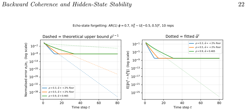
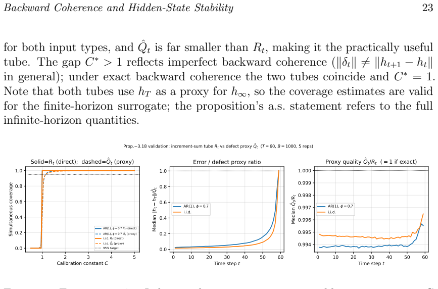
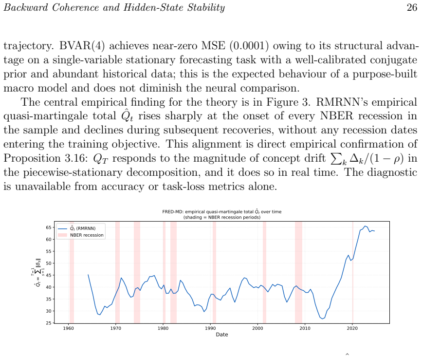
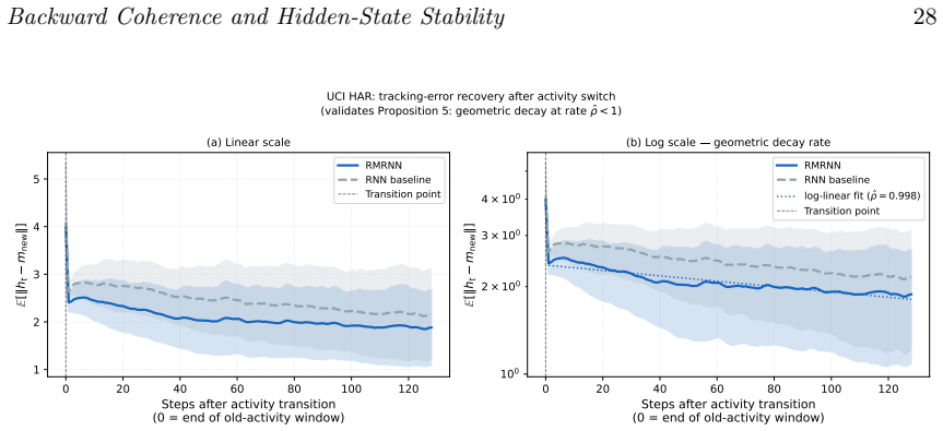
Recurrent neural networks maintain a hidden state $h_t$, but its probabilistic meaning is often unclear. We study hidden-state stability through \emph{backward coherence}: the extent to which $h_t$ can be reconstructed from $h_{t+1}$ by a learned backward projector $g_\phi$. Under contraction and summable backward drift, the hidden-state sequence forms a quasi-reverse-martingale. This yields almost-sure convergence, rates under mixing, an interpretable limiting representation, finite pathwise stopping times, and a theoretical framework for time-uniform confidence sequences. Simulations support the theory. Backward-coherence regularisation reduces the empirical quasi-martingale total $\hat Q$ by $43$--$58%$, reaches stability $28$--$44%$ earlier than an unregularised RNN, and gives tracking-error recovery consistent with geometric bounds. Additional tests confirm echo-state forgetting rates bounded by $\rho$ and verify the increment-sum tube $R_t$ with $100%$ simultaneous coverage, although $R_t$ is conservative; in practice, the defect-tail proxy $\hat Q_t$ is the more useful monitor. The backward-coherence loss is also equivalent to minimising a Kullback--Leibler divergence in a Gaussian backward model, linking the method to variational inference. Extensions cover $\phi$-mixing inputs, change-point tracking, and finite-sample concentration. Three real-data studies further validate the approach. On PhysioNet 2012 ICU data, the Reverse Martingale RNN (RMRNN) matches RNN mortality-prediction AUC while reaching stable representations 13 hours earlier. On FRED-MD, it reduces one-month-ahead forecast error by about fourfold under concept drift. On UCI Human Activity Recognition, it maintains lower post-transition tracking error with geometric decay. The guarantees apply under the stated assumptions; universality is not claimed.
Editorial analysis
A structured set of objections, weighed in public.
Referee Report
Summary. The manuscript develops a quasi-reverse-martingale theory for RNN hidden-state stability based on backward coherence, implemented via a learned backward projector g_φ. Under stated contraction and summable backward-drift conditions, the hidden-state sequence is shown to form a quasi-reverse-martingale, yielding almost-sure convergence, mixing rates, an interpretable limit, finite pathwise stopping times, and time-uniform confidence sequences. Simulations demonstrate that backward-coherence regularization reduces the empirical quasi-martingale total by 43–58%, accelerates stability, and produces tracking-error decay consistent with geometric bounds; real-data experiments on PhysioNet 2012, FRED-MD, and UCI HAR show comparable predictive performance with earlier stability or reduced post-drift error.
Significance. If the contraction and drift assumptions hold for the fitted projector, the work supplies a conditional but non-tautological theoretical framework that connects RNN dynamics to martingale convergence and stopping-time results, together with a regularization method whose loss is equivalent to a Gaussian KL objective. The explicit non-universality statement and the provision of both synthetic verification (echo-state bounds, R_t coverage) and three real-world concept-drift tasks constitute concrete strengths.
minor comments (3)
- [Abstract, §3] Abstract and §3: the precise definition of the backward projector g_φ, the contraction constant, and the summable-drift condition should be stated with equation numbers so that the quasi-reverse-martingale property can be checked directly from the text.
- [Simulations] Simulation section: the statement that R_t achieves 100% simultaneous coverage should indicate whether this is a theoretical guarantee under the stated assumptions or an empirical observation, and the coverage level should be specified.
- [Real-data studies] Real-data experiments: the precise architecture, training protocol, and hyper-parameter ranges used for the RMRNN versus baseline RNN should be reported to allow reproduction of the reported AUC, forecast-error, and stability-time improvements.
Simulated Author's Rebuttal
We thank the referee for the positive and constructive review, including the detailed summary of the quasi-reverse-martingale framework, empirical results, and recommendation for minor revision. No specific major comments were raised in the report, so we have no points requiring point-by-point rebuttal at this stage. We are happy to incorporate any minor editorial or clarification changes suggested during the revision process.
Circularity Check
No significant circularity; derivation is conditional on explicit assumptions
full rationale
The paper derives the quasi-reverse-martingale property and its consequences (a.s. convergence, rates, stopping times, confidence sequences) explicitly from the contraction mapping and summable backward-drift conditions on the learned backward projector g_φ. These are stated as assumptions under which the guarantees hold, with no claim of universality or that the properties hold unconditionally. The projector is fitted in practice, but the theoretical claims do not reduce to tautologies or rename the fit as a prediction; empirical results are presented separately as consistent with the conditional theory. No self-citation load-bearing steps, self-definitional reductions, or ansatz smuggling appear in the provided abstract or described chain. The derivation is therefore self-contained given its premises.
Axiom & Free-Parameter Ledger
free parameters (1)
- backward projector parameters φ
axioms (1)
- domain assumption The hidden-state sequence satisfies contraction and summable backward drift.
invented entities (2)
-
backward projector g_φ
no independent evidence
-
quasi-reverse-martingale
no independent evidence
Reference graph
Works this paper leans on
-
[1]
Bengio, Y., Simard, P., and Frasconi, P. (1994). Learning long-term dependencies with gradient descent is difficult.IEEE Transactions on Neural Networks,5(2), 157–166
1994
-
[2]
M., Kucukelbir, A., and McAuliffe, J
Blei, D. M., Kucukelbir, A., and McAuliffe, J. D. (2017). Variational inference: a review for statisticians.Journal of the American Statistical Association,112(518), 859–877
2017
-
[3]
Bradley, R. C. (2007).Introduction to Strong Mixing Conditions, Vols. 1–3. Kendrick
2007
-
[4]
Cho, K., van Merrienboer, B., G¨ ul¸ cehre,C ¸., Bahdanau, D., Bougares, F., Schwenk, H., and Bengio, Y. (2014). Learning phrase representations using RNN encoder– decoder for statistical machine translation. InProceedings of the 2014 Conference on Empirical Methods in Natural Language Processing (EMNLP), pp. 1724–1734
2014
-
[5]
C., and Bengio, Y
Chung, J., Kastner, K., Dinh, L., Goel, K., Courville, A. C., and Bengio, Y. (2015). A recurrent latent variable model for sequential data. InAdvances in Neural Information Processing Systems 28, pp. 2980–2988
2015
-
[6]
Doob, J. L. (1953).Stochastic Processes. Wiley, New York
1953
-
[7]
(2019).Probability: Theory and Examples, 5th ed
Durrett, R. (2019).Probability: Theory and Examples, 5th ed. Cambridge University
2019
-
[8]
Elman, J. L. (1990). Finding structure in time.Cognitive Science,14(2), 179–211
1990
-
[9]
B., Azencot, O., Queiruga, A., Hodgkinson, L., and Mahoney, M
Erichson, N. B., Azencot, O., Queiruga, A., Hodgkinson, L., and Mahoney, M. W. (2021). Lipschitz recurrent neural networks. InProceedings of the 9th International Conference on Learning Representations (ICLR)
2021
-
[10]
K., Paquet, U., and Winther, O
Fraccaro, M., Sønderby, S. K., Paquet, U., and Winther, O. (2016). Sequential neural models with stochastic layers. InAdvances in Neural Information Processing Systems 29, pp. 2199–2207
2016
-
[11]
Gama, J., ˇZliobait˙ e, I., Bifet, A., Pechenizkiy, M., and Bouchachia, A. (2014). A survey on concept drift adaptation.ACM Computing Surveys,46(4), 44:1–44:37
2014
-
[12]
He, K., Zhang, X., Ren, S., and Sun, J. (2016). Deep residual learning for image recognition. InProceedings of the IEEE Conference on Computer Vision and Pattern Recognition (CVPR), pp. 770–778
2016
-
[13]
and Schmidhuber, J
Hochreiter, S. and Schmidhuber, J. (1997). Long short-term memory.Neural Com- putation,9(8), 1735–1780
1997
-
[14]
R., Ramdas, A., McAuliffe, J., and Sekhon, J
Howard, S. R., Ramdas, A., McAuliffe, J., and Sekhon, J. (2021). Time-uniform, nonparametric, nonasymptotic confidence sequences.Annals of Statistics,49(2), 1055–1080
2021
-
[15]
echo state
Jaeger, H. (2001). The “echo state” approach to analysing and training recurrent neu- ral networks.GMD Report148. German National Research Center for Information
2001
-
[16]
Khalil, H. K. (2002).Nonlinear Systems, 3rd ed. Prentice Hall, Upper Saddle River, NJ
2002
-
[17]
Krickeberg, K. (1956). Convergence of martingales with a directed index set.Trans- actions of the American Mathematical Society,83(2), 313–337
1956
-
[18]
Kushner, H. J. and Yin, G. G. (2003).Stochastic Approximation and Recursive Algorithms and Applications, 2nd ed. Springer, New York
2003
-
[19]
McDiarmid, C. (1989). On the method of bounded differences. InSurveys in Combi- natorics, London Mathematical Society Lecture Notes 141, pp. 148–188. Cambridge University Press, Cambridge
1989
-
[20]
and Tweedie, R
Meyn, S. and Tweedie, R. L. (2009).Markov Chains and Stochastic Stability, 2nd ed. Cambridge University Press, Cambridge
2009
-
[21]
and Hardt, M
Miller, J. and Hardt, M. (2019). Stable recurrent models. InProceedings of the 7th International Conference on Learning Representations (ICLR)
2019
-
[22]
Miyato, T., Kataoka, T., Koyama, M., and Yoshida, Y. (2018). Spectral normaliza- tion for generative adversarial networks. InProceedings of the 6th International Conference on Learning Representations (ICLR)
2018
-
[23]
(1975).Discrete Parameter Martingales
Neveu, J. (1975).Discrete Parameter Martingales. North-Holland, Amsterdam
1975
-
[24]
Opial, Z. (1967). Weak convergence of the sequence of successive approximations for nonexpansive mappings.Bulletin of the American Mathematical Society,73(4), 591–597
1967
-
[25]
Pascanu, R., Mikolov, T., and Bengio, Y. (2013). On the difficulty of training recurrent neural networks. InProceedings of the 30th International Conference on Machine Learning (ICML), pp. 1310–1318
2013
-
[26]
Rajpurkar, P., Chen, E., Banerjee, O., and Topol, E. J. (2022). AI in health and medicine.Nature Medicine,28(1), 31–38
2022
-
[27]
Rao, K. M. (1969). Quasi-martingales.Mathematica Scandinavica,24, 79–92
1969
-
[28]
Sharma, A., Nemati, S., and Clifford, G. D. (2020). Early prediction of sepsis from clinical data.Critical Care Medicine,48(2), 210–217
2020
-
[29]
(2017).Asymptotic Theory of Weakly Dependent Random Processes
Rio, E. (2017).Asymptotic Theory of Weakly Dependent Random Processes. Springer, Berlin
2017
-
[30]
and Monro, S
Robbins, H. and Monro, S. (1951). A stochastic approximation method.Annals of Mathematical Statistics,22(3), 400–407. S¨ arkk¨ a, S. (2013).Bayesian Filtering and Smoothing. Cambridge University Press, Cambridge
1951
-
[31]
and Paliwal, K
Schuster, M. and Paliwal, K. K. (1997). Bidirectional recurrent neural networks. IEEE Transactions on Signal Processing,45(11), 2673–2681. Backward Coherence and Hidden-State Stability33
1997
-
[32]
Shumway, R. H. and Stoffer, D. S. (2000).Time Series Analysis and Its Applications
2000
-
[33]
N., Kaiser, L., and Polosukhin, I
Vaswani, A., Shazeer, N., Parmar, N., Uszkoreit, J., Jones, L., Gomez, A. N., Kaiser, L., and Polosukhin, I. (2017). Attention is all you need. InAdvances in Neural Information Processing Systems 30, pp. 5998–6008
2017
-
[34]
Waudby-Smith, I. and Ramdas, A. (2023). Estimating means of bounded random variables by betting.Journal of the Royal Statistical Society: Series B,85(1), 1–26. doi:10.1093/jrsssb/qkac007
-
[35]
X., Doshi-Velez, F., Jung, K., Heller, K., Kale, D., Saeed, M., et al
Wiens, J., Saria, S., Sendak, M., Ghassemi, M., Liu, V. X., Doshi-Velez, F., Jung, K., Heller, K., Kale, D., Saeed, M., et al. (2019). Do no harm: a roadmap for responsible machine learning for health care.Nature Medicine,25(9), 1337–1340
2019
-
[36]
(1991).Probability with Martingales
Williams, D. (1991).Probability with Martingales. Cambridge University Press, Cambridge
1991
-
[37]
and Reyes-Ortiz, J.L
Anguita, D., Ghio, A., Oneto, L., Parra, X. and Reyes-Ortiz, J.L. (2013). A public domain dataset for human activity recognition using smartphones.Proceedings of the European Symposium on Artificial Neural Networks, Computational Intelligence and Machine Learning (ESANN), 437–442. Ba´ nbura, M., Giannone, D. and Reichlin, L. (2010). Large Bayesian vector ...
2013
-
[38]
and Ng, S
McCracken, M.W. and Ng, S. (2016). FRED-MD: a monthly database for macroeco- nomic research.Journal of Business and Economic Statistics,34, 574–589
2016
-
[39]
and Mark, R.G
Silva, I., Moody, G., Scott, D.J., Celi, L.A. and Mark, R.G. (2012). Predicting in-hospital mortality of ICU patients: the PhysioNet/Computing in Cardiology Challenge 2012.Computing in Cardiology,39, 245–248
2012
-
[40]
R., Goyal, A., Bengio, Y., Larochelle, H., Courville, A
Krueger, D., Maharaj, T., Kram´ ar, J., Pezeshki, M., Ballas, N., Ke, N. R., Goyal, A., Bengio, Y., Larochelle, H., Courville, A. and Pal, C. (2017). Zoneout: Regu- larizing RNNs by randomly preserving hidden activations. InProceedings of the International Conference on Learning Representations (ICLR 2017)
2017
discussion (0)
Sign in with ORCID, Apple, or X to comment. Anyone can read and Pith papers without signing in.