pith. sign in

arxiv: 2606.11057 · v1 · pith:3SK6KQDVnew · submitted 2026-06-09 · 💻 cs.LG · q-bio.BM· stat.ML

Flexible Kernels for Protein Property Prediction

Pith reviewed 2026-06-27 14:13 UTC · model grok-4.3

classification 💻 cs.LG q-bio.BMstat.ML
keywords protein property predictionGaussian processessequence kernelsevolutionary substitution matricesmulti-task learningstructural conditioningdata efficiency
0
0 comments X

The pith

Sequence kernels from evolutionary matrices and local linearity yield data-efficient Gaussian processes for protein properties.

A machine-rendered reading of the paper's core claim, the machinery that carries it, and where it could break.

The paper introduces sequence kernels that draw on evolutionary substitution matrices together with local linearity to build Gaussian process models of protein landscapes. These models are shown to work well with sparse experimental data on properties such as binding affinity and thermostability. The kernels can be extended to incorporate structural information, enabling multi-task learning across different protein properties and outperforming both embedding-based baselines and purely local supervised methods.

Core claim

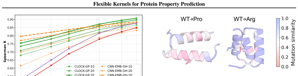
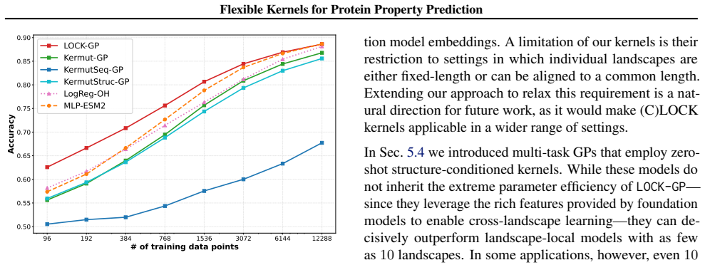
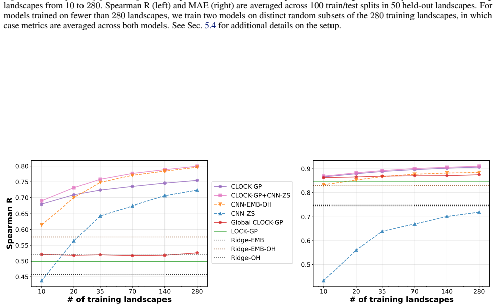
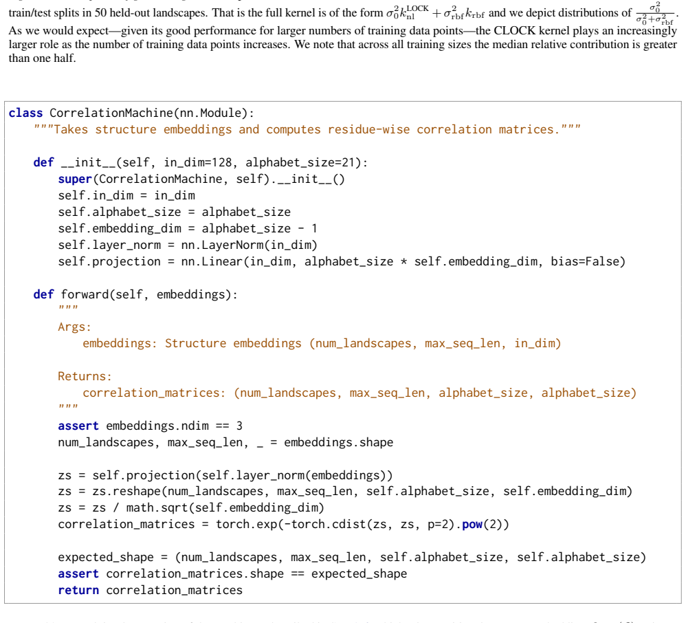
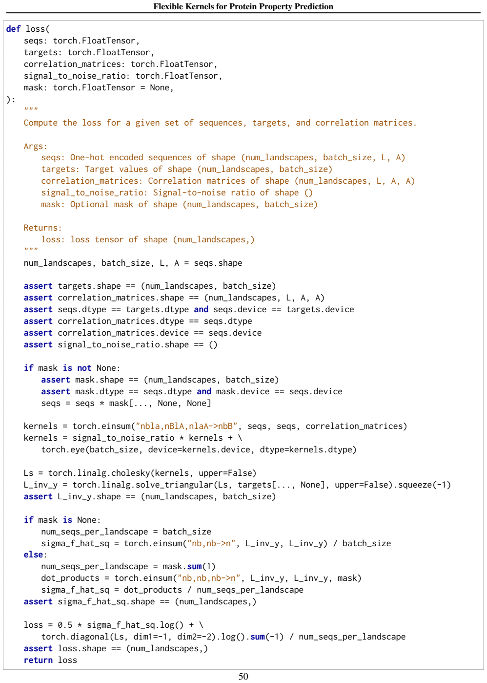
We introduce a class of sequence kernels that exploit evolutionary substitution matrices as well as local linearity and demonstrate that the resulting Gaussian processes provide data-efficient models of protein property landscapes, frequently outperforming alternatives that rely on foundation model embeddings. Furthermore--by learning what are in effect structure-aware substitution matrices--we show that our kernels can readily incorporate structural information from foundation models. We demonstrate that these structure-conditioned kernels are well suited to multi-task learning across multiple protein property landscapes and can decisively outperform local supervised learning methods.

What carries the argument

Sequence kernels that combine evolutionary substitution matrices with local linearity, which can be conditioned on structural data to learn structure-aware substitution matrices.

Load-bearing premise

Kernels built from evolutionary substitution matrices plus local linearity generalize across protein families and properties without requiring extensive hyperparameter tuning or suffering from distribution shift when applied to new sequences.

What would settle it

A comparison on held-out protein families or properties where the Gaussian process models built from these kernels fail to match or exceed the predictive accuracy or data efficiency of foundation-model embedding baselines.

Figures

Figures reproduced from arXiv: 2606.11057 by Gevorg Grigoryan, Henry N. Ward, Hunter Nisonoff, James M. McFarland, Martin Jankowiak, Rudraksh Tuwani, Yerdos Ordabayev.

Figure 1
Figure 1. Figure 1: The BLOSUM50 substitution matrix as a correlation matrix. We zoom-in on four amino acids, two of which are bio￾physically similar (valine and isoleucine) and two of which are largely dissimilar to all other amino acids (tryptophan and cys￾teine). The matrix on the right has been raised to the power 0.03. For details on the normalization scheme we use refer to Sec. A.3. For the full matrix see [PITH_FULL_I… view at source ↗
Figure 2
Figure 2. Figure 2: Predictive performance as a function of the number of training data points in the cross-validation setting. We depict Pearson R (left) and mean absolute error (right); metrics are averaged across 21 datasets. See Sec. 5.3 for discussion and [PITH_FULL_IMAGE:figures/full_fig_p006_2.png] view at source ↗
Figure 3
Figure 3. Figure 3: Predictive performance of GP models as a function of the number of training data points in the cross-validation setting. We depict the continuous ranked probability score (CRPS; Gneiting & Raftery (2007)), an MAE-like proper scoring rule that evaluates both accuracy and calibration of predictive distributions. Metrics are averaged across 21 datasets. residuewise exponents αℓ improves fit noticeably; and v)… view at source ↗
Figure 4
Figure 4. Figure 4: Predictive performance as a function of the number of (landscape-local) training data points on the multi-landscape thermostability data described in Sec. 5.4. We depict both Spear￾man R (top) and mean absolute error (bottom); metrics are aver￾aged across 100 train/test splits in 50 held-out landscapes. The structure-conditioned CLOCK-GP augmented with an additional CNN-based kernel performs best across th… view at source ↗
Figure 6
Figure 6. Figure 6: Structure-conditioned amino acid correlations learned by CLOCK on representative structures from Tsuboyama et al. (2023). Left (PDB ID: 2JVD): correlation between the wild-type amino acid and proline at each position. Right (PDB ID: 2JWD): correlation between the wild-type amino acid and arginine. Each structure highlights a pair of sites (namely those with sidechains pictured) with the same amino-acid ide… view at source ↗
Figure 7
Figure 7. Figure 7: We report binary classification accuracy for models trained on (quantized) fluorescence readouts from Gonzalez Somer￾meyer et al. (2022) as a function of the number of training data points. Accuracy is averaged across three replicates. LogReg-OH is logistic regression on one-hot features and is the direct analog of Ridge-OH in Sec. 5.3. 5.5. Thompson Sampling We demonstrate the utility of LOCK-GP uncertain… view at source ↗
Figure 8
Figure 8. Figure 8: We depict results for the Thompson sampling experiment in Sec. A.6. Solid lines depict properties of the sequences obtained from solving Eqn. 26 at five distinct concentrations α; uncertainty bands reflect standard errors. Dashed lines depict properties of the sequences obtained from solving Eqn. 25, which corresponds to the α → ∞ limit. We average across 10 replicate experiments. As the concentration α go… view at source ↗
Figure 9
Figure 9. Figure 9: Structure-conditioned amino acid correlations learned by the CLOCK kernel. We show representative structures from Tsuboyama et al. (2023), coloring the wild-type residue at each position by its CLOCK correlation Cℓaaref (Eqn. 14) to one of three reference amino acids (Pro, Arg, Gly; rows). Each structure highlights a pair of sites (namely those with sidechains pictured) with the same amino-acid identity bu… view at source ↗
Figure 10
Figure 10. Figure 10: We compare several GPs trained on the AAV dataset from Sinai et al. (2021). We plot both Spearman R (left) and MAE (right); metrics are averaged across 10 i.i.d. train/test splits. All GPs are CLOCK-GPs except for the BLOSUM GP, which uses the same correlation matrix at each position. All CLOCK-GPs use a W tensor (see Eqn. 15) that is pre-trained on thermostability data (see Sec. 5.4). All CLOCK-GPs apart… view at source ↗
Figure 11
Figure 11. Figure 11: We compare several GPs trained on the AAV dataset from Sinai et al. (2021). We plot both Pearson R (left) and RMSE (right); metrics are averaged across 10 i.i.d. train/test splits. All GPs are CLOCK-GPs except for the BLOSUM GP, which uses the same correlation matrix at each position. All CLOCK-GPs use a W tensor (see Eqn. 15) that is pre-trained on thermostability data (see Sec. 5.4). All CLOCK-GPs apart… view at source ↗
Figure 12
Figure 12. Figure 12: We report Spearman R for models trained on the amacGFP dataset from Gonzalez Somermeyer et al. (2022) as a function of the number of training data points. Spearman R is averaged across three replicates. Apart from the binary classification experiment in Sec. 5.6, the GP experiments in Sec. 5 focus on the regression setting with small-to-moderate sized datasets, a regime in which exact inference is viable.… view at source ↗
Figure 13
Figure 13. Figure 13: We depict Spearman R metrics obtained for 8 ProteinGym datasets for all three Kermut variants, comparing our implementation to the results provided by Groth et al. (2024). The number in parentheses after each landscape indicates the total number of data points in the given landscape. since the sum that defines kstruct(x (ℓ) , x (ℓ+1)) contains all the terms that enter into kstruct(x (ℓ−1) , x (ℓ) ) plus n… view at source ↗
Figure 14
Figure 14. Figure 14: Predictive performance as a function of the number of training data points in the cross-validation setting. We depict Spearman R (left) and RMSE (right); metrics are averaged across 21 datasets. See Sec. 5.3 for discussion and Sec. A.16.1 for details on each model. Landscape LOCK-GP Tanimoto-GP MLP-ESM2-LastLayer Kermut-GP KermutSeq-GP KermutStruc-GP Ridge-ESM2 Ridge-OH SigGLM-OH BLOSUM50-ZeroShot ESM2-65… view at source ↗
Figure 15
Figure 15. Figure 15: [Companion figure to Fig [PITH_FULL_IMAGE:figures/full_fig_p043_15.png] view at source ↗
Figure 16
Figure 16. Figure 16: The BLOSUM50 substitution matrix normalized as a 21×21 correlation matrix. See Sec. A.3.1 for details on the normalization scheme used. We include the gap token ‘-’. The correlation ranges from 0.59 to 1.0. 43 [PITH_FULL_IMAGE:figures/full_fig_p043_16.png] view at source ↗
Figure 17
Figure 17. Figure 17: The global correlation matrix fit to the thermostability data described in Sec. 5.4. We include the gap token ‘-’. The correlation ranges from 0.06 to 1.0. A C D E F G H I K L M N P Q R S T V W Y - A C D E F G H I K L M N P Q R S T V W Y - 0.0 0.2 0.4 0.6 0.8 1.0 [PITH_FULL_IMAGE:figures/full_fig_p044_17.png] view at source ↗
Figure 18
Figure 18. Figure 18: A visual representation of the CLOCK-GP correlation matrix fit to the thermostability data described in Sec. 5.4. Since the correlation matrix varies from position to position, we depict the average correlation matrix across all positions in the 50 held-out test landscapes. We include the gap token ‘-’. The correlation ranges from 0.63 to 1.0. 44 [PITH_FULL_IMAGE:figures/full_fig_p044_18.png] view at source ↗
Figure 19
Figure 19. Figure 19: [Companion figure to [PITH_FULL_IMAGE:figures/full_fig_p045_19.png] view at source ↗
Figure 20
Figure 20. Figure 20: [Companion figure to Fig [PITH_FULL_IMAGE:figures/full_fig_p045_20.png] view at source ↗
Figure 21
Figure 21. Figure 21: [Companion figure to Fig [PITH_FULL_IMAGE:figures/full_fig_p046_21.png] view at source ↗
Figure 22
Figure 22. Figure 22: [Companion figure to Fig [PITH_FULL_IMAGE:figures/full_fig_p046_22.png] view at source ↗
Figure 23
Figure 23. Figure 23: [Companion figure to Fig [PITH_FULL_IMAGE:figures/full_fig_p046_23.png] view at source ↗
Figure 24
Figure 24. Figure 24: [Companion figure to Fig [PITH_FULL_IMAGE:figures/full_fig_p047_24.png] view at source ↗
Figure 25
Figure 25. Figure 25: [Companion figure to Fig [PITH_FULL_IMAGE:figures/full_fig_p047_25.png] view at source ↗
Figure 26
Figure 26. Figure 26: [Companion figure to Fig [PITH_FULL_IMAGE:figures/full_fig_p048_26.png] view at source ↗
Figure 27
Figure 27. Figure 27: [Companion figure to Fig [PITH_FULL_IMAGE:figures/full_fig_p048_27.png] view at source ↗
Figure 28
Figure 28. Figure 28: [Companion figure to Fig [PITH_FULL_IMAGE:figures/full_fig_p048_28.png] view at source ↗
Figure 29
Figure 29. Figure 29: [Companion figure to Fig [PITH_FULL_IMAGE:figures/full_fig_p049_29.png] view at source ↗
Figure 30
Figure 30. Figure 30: Pytorch implementation of the machinery described in Sec. 3.6, which takes positional structure embeddings h1:L(S) as input and returns correlation matrices C1:L. 49 [PITH_FULL_IMAGE:figures/full_fig_p049_30.png] view at source ↗
Figure 31
Figure 31. Figure 31: Pytorch implementation of the concentration-likelihood-based training loss used in CLOCK. See Sec. A.8 for details. 50 [PITH_FULL_IMAGE:figures/full_fig_p050_31.png] view at source ↗
read the original abstract

Despite its importance to applications in protein design, predicting protein properties like binding affinity and thermostability from sparse experimental data remains a significant challenge. Accordingly, we introduce a class of sequence kernels that exploit evolutionary substitution matrices as well as local linearity and demonstrate that the resulting Gaussian processes provide data-efficient models of protein property landscapes, frequently outperforming alternatives that rely on foundation model embeddings. Furthermore--by learning what are in effect structure-aware substitution matrices--we show that our kernels can readily incorporate structural information from foundation models. We demonstrate that these structure-conditioned kernels are well suited to multi-task learning across multiple protein property landscapes and can decisively outperform local supervised learning methods.

Editorial analysis

A structured set of objections, weighed in public.

Desk editor's note, referee report, simulated authors' rebuttal, and a circularity audit. Tearing a paper down is the easy half of reading it; the pith above is the substance, this is the friction.

Referee Report

0 major / 1 minor

Summary. The manuscript introduces a class of sequence kernels for Gaussian processes that exploit evolutionary substitution matrices together with local linearity to model protein property landscapes from sparse data. It further shows how these kernels can be conditioned on structural information from foundation models by learning structure-aware substitution matrices. The central empirical claims are that the resulting GPs are data-efficient and frequently outperform alternatives based on foundation model embeddings, and that the structure-conditioned kernels are particularly well-suited to multi-task learning across multiple protein properties, where they can decisively outperform local supervised learning methods.

Significance. If the reported performance gains are robust, the work would offer a useful kernel-based alternative to embedding-heavy approaches for low-data protein property prediction tasks such as binding affinity and thermostability. The explicit incorporation of evolutionary priors and the multi-task capability are strengths that could reduce reliance on large foundation models while remaining computationally tractable. The approach appears to operate with few or no free parameters beyond the kernel construction itself.

minor comments (1)
  1. [Abstract] Abstract: the strong claims of frequent outperformance and decisive multi-task gains would be easier to evaluate if the abstract briefly indicated the protein families, number of properties/tasks, and evaluation protocol used.

Simulated Author's Rebuttal

0 responses · 0 unresolved

We thank the referee for the positive assessment of our manuscript and the recommendation for minor revision. The summary accurately reflects the core contributions regarding sequence kernels that leverage substitution matrices and local linearity for data-efficient Gaussian process modeling of protein properties, as well as the structure-aware extensions for multi-task learning.

Circularity Check

0 steps flagged

No significant circularity identified

full rationale

The provided abstract and context describe an empirical introduction of sequence kernels exploiting substitution matrices and local linearity, with Gaussian process performance claims presented as experimental outcomes on protein property data. No derivation chain, equations, or self-citations are visible that reduce predictions to fitted inputs by construction, self-definitional loops, or load-bearing self-citations. The central claims rest on outperformance demonstrations rather than tautological redefinitions, making the work self-contained against external benchmarks with no circular steps exhibited.

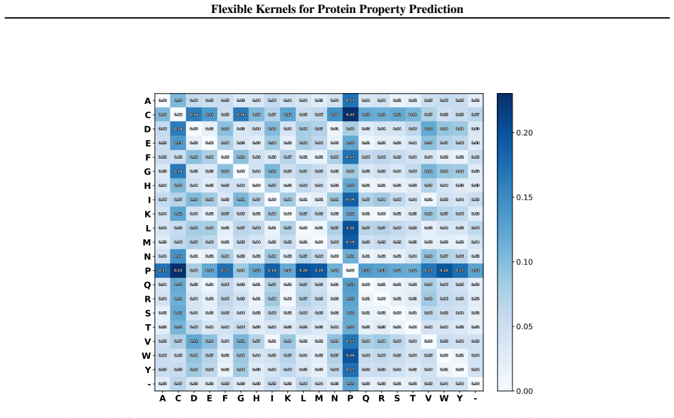
Axiom & Free-Parameter Ledger

0 free parameters · 0 axioms · 0 invented entities

Abstract-only review provides no concrete information on free parameters, axioms, or invented entities; all fields left empty.

pith-pipeline@v0.9.1-grok · 5663 in / 987 out tokens · 20021 ms · 2026-06-27T14:13:25.684829+00:00 · methodology

discussion (0)

Sign in with ORCID, Apple, or X to comment. Anyone can read and Pith papers without signing in.

Reference graph

Works this paper leans on

13 extracted references · 3 canonical work pages

  1. [1]

    URL http: //dx.doi.org/10.1038/s41467-024-45621-4

    doi: 10.1038/s41467-024-45621-4. URL http: //dx.doi.org/10.1038/s41467-024-45621-4. Elnaggar, A., Heinzinger, M., Dallago, C., Rehawi, G., Wang, Y ., Jones, L., Gibbs, T., Feher, T., Angerer, C., Steinegger, M., Bhowmik, D., and Rost, B. Prottrans: Toward understanding the language of life through self- supervised learning.IEEE Transactions on Pattern Ana...

  2. [2]

    Highly accurate protein structure prediction with

    doi: 10.1038/s41586-021-03819-2. Khan, A., Cowen-Rivers, A. I., Grosnit, A., Deik, D.-G.- X., Robert, P. A., Greiff, V ., Smorodina, E., Rawat, P., Akbar, R., Dreczkowski, K., et al. Toward real-world automated antibody design with combinatorial bayesian optimization.Cell Reports Methods, 3(1), 2023. Koshi, J. M. and Goldstein, R. A. Context-dependent opt...

  3. [3]

    doi: 10.7554/elife.83442

    ISSN 2050-084X. doi: 10.7554/elife.83442. URL http://dx.doi.org/10.7554/eLife.83442. Notin, P., Kollasch, A., Ritter, D., Van Niekerk, L., Paul, S., Spinner, H., Rollins, N., Shaw, A., Orenbuch, R., Weitz- man, R., et al. Proteingym: Large-scale benchmarks for protein fitness prediction and design.Advances in Neu- ral Information Processing Systems, 36:64...

  4. [4]

    for everyt >0, the kernelk t(i, j) = exp −t ψ(i, j) is positive semidefinite

  5. [5]

    for finite index sets,ψis a squared Euclidean distance. A.1.2. CHARACTERIZINGINFINITELYDIVISIBLEMATRICES With these definitions in hand, we can give a precise characterization of infinitely divisible matrices. Lemma A.8(Berg et al. (1984)).Let K be a symmetric matrix with strictly positive entries. Then K is infinitely divisible if and only iflog ◦ Kiscon...

  6. [6]

    linear kernel plus non-linear kernel times linear kernel

    There exist pointsx 1, . . . , xA inR m (for somem≤A−1) such that Kij = exp − ∥xi −x j∥2 for alli, j. In particular, every infinitely divisible correlation matrix is of the formK= exp ◦(−D) where D is asquared Euclidean distance matrix. Proof. By Lemma A.8,(1) ⇔ (2). By Schoenberg’s Theorem A.7,(2) ⇔ (3): D is CNSD iff e−tD is PSD for all t >0 , and for f...

  7. [7]

    prior on each ˜αℓ.Marginally, this choice corresponds to a LogNormal(0, 5

  8. [8]

    prior on αℓ. We note that choosing an overcomplete parameterization has an impact on theoptimization dynamics; in particular by introducing ˜αwe expect it to be easier to take larger steps in αℓ space. These priors were chosen based on regression experiments conducted with datasets disjoint from those used in our experiments in Sec. 5. A.4. Epistasis and ...

  9. [9]

    non-unique) sequences

    it heavily penalizes sets of sequencesx 1:N that contain duplicate (i.e. non-unique) sequences

  10. [10]

    catastrophic NLL

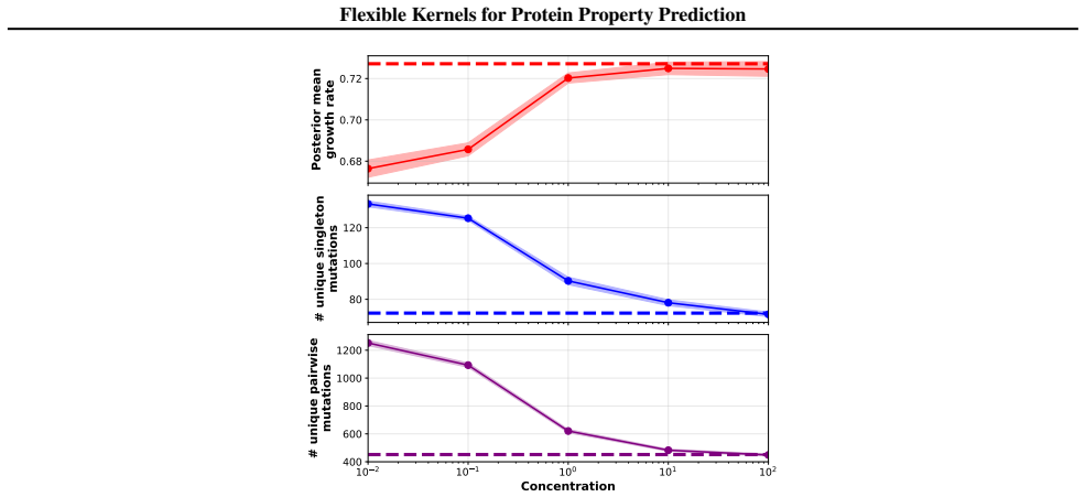
    it strongly encourages the sequences x1:N to spread out in a balanced manner across a nested set of 8 Hamming shells centered around the wild-type sequencex wt In particular Ψ(x1:N) strongly encourages exactly 100 of the 800 sequences to reside in the2-Hamming shell of xwt, exactly 100 of the 800 sequences to reside in the 3-Hamming shell of xwt, and so o...

  11. [11]

    PLM UsageESM-2 and ESM-1v were pre-trained on single chain sequences, while some of our datasets consist of multi-chain proteins

    is used instead of ESM-2-8M. PLM UsageESM-2 and ESM-1v were pre-trained on single chain sequences, while some of our datasets consist of multi-chain proteins. Therefore, when computing ESM-2 embeddings or fine-tuning ESM-1v we proceed as follows. For each sequence we: i) obtain the chain boundaries from the associated reference structure; ii) compute inde...

  12. [12]

    By contrast BLOSUM50-based zero-shot scores are consistently positive except for the two thermostability landscapes from Tsuboyama et al

    for similar observations. By contrast BLOSUM50-based zero-shot scores are consistently positive except for the two thermostability landscapes from Tsuboyama et al. (2023) and some of the antibody landscapes from Moulana et al. (2023). Swapping ESM2-8M for ESM-650M in ridge regression and MLP models has mixed effects on performance. While Ridge-ESM2-650M o...

  13. [13]

    training set

    Metrics are averaged across 21 datasets. For each column the best performing metric is marked in bold. This table is identical to Table 1, except that it contains additional models (marked in purple). We do not include MAE metrics for zero-shot methods, since they are wildly off-scale. Note that Ridge-ESM2-8M is referred to as Ridge-ESM2 in the main text....