Holonomy Analysis of Optical-polarization Temperature Trajectories in Stress-induced Ferroelectric SrTiO₃
Pith reviewed 2026-06-27 06:11 UTC · model grok-4.3
The pith
Holonomies from temperature trajectories in optical polarization data diagnose electromechanical inhomogeneity in stressed SrTiO3 without reconstructing internal fields.
A machine-rendered reading of the paper's core claim, the machinery that carries it, and where it could break.
Core claim
By casting optical-polarization responses as temperature trajectories and using SVD to separate direction structure and evolution modes, holonomies computed by transporting these objects around closed real-space loops produce maps of connection mismatches that are spatially localized and correlated with enhanced ferroelectric transition temperature and stress-related optical anisotropy in SrTiO3, distinct from orientational disorder and simple spatial variation, with signed holonomy resolving positive and negative structures.
What carries the argument
Holonomies obtained by transporting SVD-derived optical-polarization-direction structure and temperature-evolution modes around closed loops in real space, providing a measure of connection mismatches.
If this is right
- Holonomy maps identify regions with enhanced ferroelectric transition temperature under stress.
- The signed holonomy of temperature-evolution modes distinguishes positive and negative connection structures under a fixed frame.
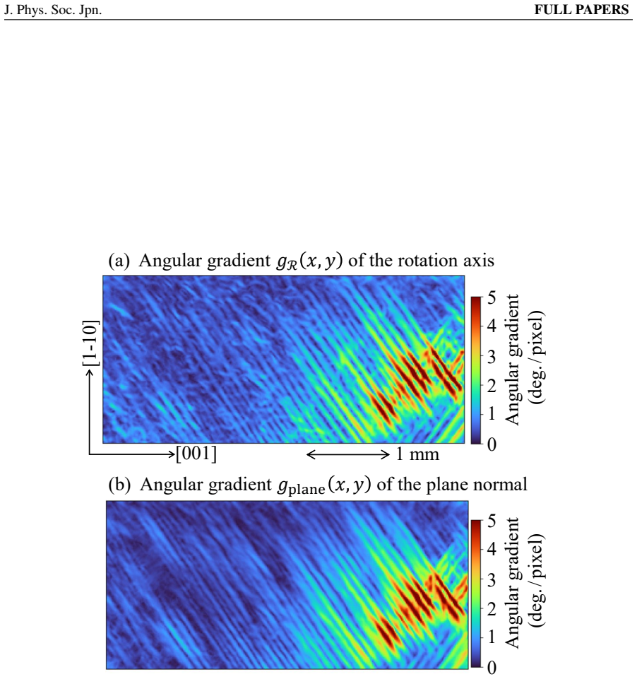
- Local order parameter and angular-gradient analyses confirm holonomy signals differ from orientational disorder or simple spatial variation.
- The framework provides an experimentally accessible diagnostic for electromechanical inhomogeneity via birefringence imaging data.
Where Pith is reading between the lines
- This trajectory-based geometric method on imaging data could extend to other condensed-matter systems with temperature-dependent optical responses.
- It may connect to parallel transport concepts in related physical contexts such as Berry phases in similar datasets.
- Direct comparison with controlled samples having known strain distributions would test the separation from disorder effects.
- The approach suggests potential for real-space geometric diagnostics in other forms of spatially resolved measurement data.
Load-bearing premise
The SVD-derived geometric objects from polarization trajectories can be parallel transported around closed real-space loops such that the resulting holonomy mismatches reflect physical electromechanical inhomogeneity rather than artifacts of measurement or data processing.
What would settle it
If holonomy maps show no correlation with independent local transition temperature measurements or match patterns expected from orientational disorder simulations alone, the claim that they diagnose physical inhomogeneity would be falsified.
Figures
read the original abstract
We develop a data-induced geometric framework for temperature trajectories in optical-polarization data and apply it to temperature-dependent birefringence imaging of stress-induced ferroelectric SrTiO$_3$. By treating the measured response as an observable projection of local material states, the optical-polarization response at each pixel is cast as a trajectory along the temperature axis. Singular value decomposition separates trajectory-induced geometric objects associated with optical-polarization-direction structure and temperature-evolution modes. Holonomies are then defined by transporting these objects around closed loops in real space. The resulting maps reveal spatially localized connection mismatches correlated with an enhanced ferroelectric transition temperature and stress-related optical anisotropy. Local order parameters and angular-gradient analyses confirm that these loop-level signals are distinct from orientational disorder and simple spatial variation. The signed holonomy of the temperature-evolution modes further resolves positive and negative connection structures under a fixed frame convention. These results demonstrate that the data-induced connection geometry of temperature trajectories provides an experimentally accessible diagnostic of electromechanical inhomogeneity in SrTiO$_3$ under stress, without explicitly reconstructing hidden strain or electric-polarization fields.
Editorial analysis
A structured set of objections, weighed in public.
Referee Report
Summary. The manuscript develops a data-induced geometric framework for temperature trajectories extracted from optical-polarization birefringence imaging of stress-induced ferroelectric SrTiO₃. Per-pixel temperature trajectories are decomposed via singular value decomposition into geometric objects associated with optical-polarization-direction structure and temperature-evolution modes. Holonomies are obtained by transporting these objects around closed real-space loops; the resulting maps display spatially localized connection mismatches that correlate with an enhanced ferroelectric transition temperature and stress-related optical anisotropy. Local order parameters and angular-gradient analyses are used to establish that the loop-level signals are distinct from orientational disorder and simple spatial variation. The signed holonomy of the temperature-evolution modes is shown to resolve positive and negative connection structures under a fixed frame convention. The central claim is that this data-induced connection geometry supplies an experimentally accessible diagnostic of electromechanical inhomogeneity without explicit reconstruction of hidden strain or polarization fields.
Significance. If the holonomy construction and its distinction from disorder hold, the work supplies a novel geometric diagnostic for electromechanical inhomogeneity in ferroelectrics that operates directly on imaging trajectories. The data-induced character of the method and the explicit controls via order parameters and angular gradients are strengths that differentiate it from conventional field-reconstruction approaches. The framework could be extended to other trajectory-based imaging modalities in condensed-matter materials science.
minor comments (3)
- The abstract states that local order parameters and angular-gradient analyses confirm distinction from orientational disorder, but the main text should include a dedicated paragraph or subsection (e.g., near the holonomy maps) that quantifies how these controls rule out the alternative interpretations with explicit metrics or thresholds.
- [Methods] The definition of the connection and the precise transport rule for the SVD-derived objects around real-space loops should be stated with an equation or pseudocode in the methods section to permit independent implementation.
- Figure captions for the holonomy maps should specify the loop radii or pixel counts employed and indicate whether the signed holonomy is computed in a single global frame or per-pixel frames.
Simulated Author's Rebuttal
We thank the referee for the detailed and positive assessment of our manuscript, including the recognition of the data-induced geometric framework, its distinction from conventional approaches, and the potential for extension to other imaging modalities. The recommendation for minor revision is noted; however, the report does not raise any specific major comments requiring clarification or modification.
Circularity Check
No significant circularity identified
full rationale
The paper's chain applies SVD to extract geometric objects (optical-polarization-direction structure and temperature-evolution modes) from per-pixel temperature trajectories, then defines holonomies by transporting those objects around closed real-space loops. This is a constructive, data-induced procedure whose outputs are not shown to reduce by definition to the SVD inputs or to any fitted parameters. Additional controls (local order parameters and angular-gradient analyses) are invoked to establish that the resulting mismatch signals are distinct from orientational disorder, supplying independent content. No self-citations, uniqueness theorems, or ansatzes are referenced in the provided description, and the central diagnostic claim is framed as an experimentally accessible geometric observable without explicit field reconstruction.
Axiom & Free-Parameter Ledger
axioms (1)
- standard math Singular value decomposition separates trajectory-induced geometric objects associated with optical-polarization-direction structure and temperature-evolution modes
invented entities (1)
-
Holonomies obtained by transporting SVD-derived objects around closed real-space loops
no independent evidence
Reference graph
Works this paper leans on
-
[1]
E. K. Salje,Phase transitions in ferroelastic and co-elastic crystals, (Cambridge Uni- versity Press, 1991)
1991
-
[2]
Catalan, J
G. Catalan, J. Seidel, R. Ramesh, and J. F. Scott, Rev. Mod. Phys.84, 119 (2012)
2012
-
[3]
G. Tian, W. Yang, D. Chen, Z. Fan, Z. Hou, M. Alexe, and X. Gao, Nat. Sci. Rev.6, 684 (2019)
2019
-
[4]
A. K. Tagantsev, Phys. Rev. B34, 5883 (1986)
1986
-
[5]
P. V . Yudin and A. K. Tagantsev, Nanotechnology24, 432001 (2013)
2013
-
[6]
Manaka, Y
H. Manaka, Y . Sasaki, and Y . Miura, J. Phys. Soc. Jpn.86, 114710 (2017)
2017
-
[7]
Miura, K
Y . Miura, K. Okumura, T. Fukuda, and H. Manaka, JPS Conf. Ser.969, 012153 (2018)
2018
-
[8]
Manaka, K
H. Manaka, K. Tateishi, and Y . Miura, J. Phys. Soc. Jpn.88, 124702 (2019)
2019
-
[9]
Manaka, K
H. Manaka, K. Okumura, K. Tokunaga, and Y . Miura, J. Phys. Soc. Jpn.91, 114701 (2022)
2022
-
[10]
Miura, R
Y . Miura, R. Ibushi, and H. Manaka, JPS Conf. Proc.38, 011142 (2023)
2023
-
[11]
Manaka, K
H. Manaka, K. Seike, and Y . Miura, J. Phys. Soc. Jpn.95, 063704 (2026)
2026
-
[12]
R. R. Coifman and S. Lafon, Appl. Comput. Harmon. Anal.21, 5 (2006)
2006
-
[13]
S. T. Roweis and L. K. Saul, Science290, 2323 (2000)
2000
-
[14]
Takens,Dynamical Systems and Turbulence, Proceedings of a Symposium Held at the University of Warwick 1980, p
F. Takens,Dynamical Systems and Turbulence, Proceedings of a Symposium Held at the University of Warwick 1980, p. 366 (1981)
1980
-
[15]
Uribarri and G
G. Uribarri and G. B. Mindlin, Chaos30, 093109 (2020)
2020
-
[16]
K. A. M ¨uller, W. Berlinger, and J. C. Slonczewski, Phys. Rev. Lett.25, 734 (1970)
1970
-
[17]
W. J. Burke and R. J. Pressley, Solid State Commun.9, 191 (1971)
1971
-
[18]
Sakudo and H
T. Sakudo and H. Unoki, Phys. Rev. Lett.26, 851 (1971)
1971
-
[19]
T. S. Chang, J. Appl. Phys.43, 3591 (1972)
1972
-
[20]
Uwe and T
H. Uwe and T. Sakudo, Phys. Rev. B13, 271 (1976)
1976
-
[21]
K. A. M ¨uller and H. Burkard, Phys. Rev. B19, 3593 (1979)
1979
-
[22]
Fujii, H
Y . Fujii, H. Uwe, and T. Sakudo, J. Phys. Soc. Jpn.56, 1940 (1987)
1940
-
[23]
Chrosch and E
J. Chrosch and E. K. H. Salje, J. Phys.: Condens. Matter10, 2817 (1998)
1998
-
[24]
Sidoruk, J
J. Sidoruk, J. Leist, H. Gibhardt, M. Meven, K. Hradil, and G. Eckold, J. Phys.: Condens. Matter22, 235903 (2010). 23/80 J. Phys. Soc. Jpn.FULL PAPERS
2010
-
[25]
Manaka, K
H. Manaka, K. Uetsubara, S. Korogi, and Y . Miura, J. Phys. Soc. Jpn.91, 084704 (2022)
2022
-
[26]
Manaka, K
H. Manaka, K. Uetsubara, and Y . Miura, JPS Conf. Proc.38, 011112 (2023)
2023
-
[27]
Tang and R
P. Tang and R. K. Wang, Biomed. Opt. Express11, 6852 (2020)
2020
-
[28]
Manaka, K
H. Manaka, K. Toyoda, and Y . Miura, Sci. Technol. Adv. Mater. Meth.4, 2342234 (2024)
2024
-
[29]
Machon and G
T. Machon and G. P. Alexander, Phys. Rev. X6, 011033 (2016)
2016
-
[30]
C. P. Jisha, S. Nolte, and A. Alberucci, Laser Photonics Rev.15, 2100003 (2021)
2021
-
[31]
G. H. Golub and C. F. Van Loan,Matrix Computations(Johns Hopkins University Press, Baltimore, 2013) 4th ed
2013
-
[32]
C. E. Rasmussen and C. K. I. Williams,Gaussian Processes for Machine Learning(MIT Press, Cambridge, MA, 2006)
2006
-
[33]
Mallasto and A
A. Mallasto and A. Feragen, Proc. IEEE/CVF Conf. Comput. Vis. Pattern Recognit. (CVPR), 5580 (2018)
2018
-
[34]
J. T. Wilson, V . Borovitskiy, A. Terenin, P. Mostowsky, and M. P. Deisenroth, Proc. Mach. Learn. Res.119, 10292 (2020)
2020
-
[35]
Y . Shen, J. Opt.23, 124004 (2021)
2021
-
[36]
Kuzmenko, Y
I. Kuzmenko, Y . B. Band, and Y . Avishai, Phys. Rev. B112, L020501 (2025)
2025
-
[37]
R. A. Cowley, Phys. Rev.134, A981 (1964)
1964
-
[38]
Unoki and T
H. Unoki and T. Sakudo, J. Phys. Soc. Jpn.23, 546 (1967)
1967
-
[39]
R. A. Cowley, W. J. L. Buyers, and G. Dolling, Solid State Commun.8, 181 (1969)
1969
-
[40]
Courtens, Phys
E. Courtens, Phys. Rev. Lett.29, 1380 (1972)
1972
-
[41]
Sawaguchi, A
E. Sawaguchi, A. Kikuchi, and Y . Kodera, J. Phys. Soc. Jpn.17, 1666 (1962)
1962
-
[42]
Hegenbarth, Phys
E. Hegenbarth, Phys. Status Solidi6, 333 (1964)
1964
-
[43]
P. A. Fleury and J. M. Worlock, Phys. Rev.174, 613 (1968)
1968
-
[44]
Hemberger, P
J. Hemberger, P. Lunkenheimer, R. Viana, R. B ¨ohmer, and A. Loidl, Phys. Rev. B52, 13159 (1995)
1995
-
[45]
Hemberger, M
J. Hemberger, M. Nicklas, R. Viana, P. Lunkenheimer, A. Loidl, and R. B¨ohmer, J. Phys.: Condens. Matter8, 4673 (1996)
1996
-
[46]
Manaka, H
H. Manaka, H. Nozaki, and Y . Miura, J. Phys. Soc. Jpn.86, 114702 (2017)
2017
-
[47]
Manaka, H
H. Manaka, H. Nozaki, and Y . Miura, JPS Conf. Ser.969, 012119 (2018)
2018
-
[48]
Toyoda, H
K. Toyoda, H. Manaka, and Y . Miura, Sci. Technol. Adv. Mater. Meth.3, 2278322 (2023). 24/80 J. Phys. Soc. Jpn.FULL PAPERS
2023
-
[49]
Manaka, S
H. Manaka, S. Katayama, S. Honda, and Y . Miura, Sci. Technol. Adv. Mater. Meth.5, 2568376 (2025)
2025
-
[50]
R. M. Azzam and N. M. Bashara,Ellipsometry and polarized light, (North Holland, Amsterdam, 1977)
1977
-
[51]
Manaka, G
H. Manaka, G. Yagi, and Y . Miura, Rev. Sci. Instrum.87, 073704 (2016)
2016
-
[52]
Manaka, T
H. Manaka, T. Fukuda, and Y . Miura, J. Phys. Soc. Jpn.85, 124701 (2016)
2016
-
[53]
Seike, H
K. Seike, H. Manaka, and Y . Miura, Sci. Technol. Adv. Mater. Meth.5, 2503698 (2025)
2025
-
[54]
Zubko, G
P. Zubko, G. Catalan, A. Buckley, P. R. L. Welche, and J. F. Scott, Phys. Rev. Lett.99, 167601 (2007)
2007
-
[55]
Edelman, T
A. Edelman, T. A. Arias, and S. T. Smith, SIAM J. Matrix Anal. Appl.20, 303 (1998)
1998
-
[56]
Absil, R
P.-A. Absil, R. Mahony, and R. Sepulchre,Optimization Algorithms on Matrix Manifolds (Princeton University Press, Princeton, 2008)
2008
-
[57]
Turaga, A
P. Turaga, A. Veeraraghavan, A. Srivastava, and R. Chellappa, IEEE Trans. Pattern Anal. Mach. Intell.33, 2273 (2011)
2011
-
[58]
(Supplementary Materials) [Details of the analysis methods and parameter dependence.]
-
[59]
N. I. Fisher, T. Lewis, and B. J. J. Embleton, Statistical Analysis of Spherical Data (Cam- bridge University Press, Cambridge, 1987)
1987
-
[60]
P. G. de Gennes and J. Prost,The physics of liquid crystals, (Oxford University Press, 1995)
1995
-
[61]
ref” explicitly denotes the reference series (b=1). Below, “ref
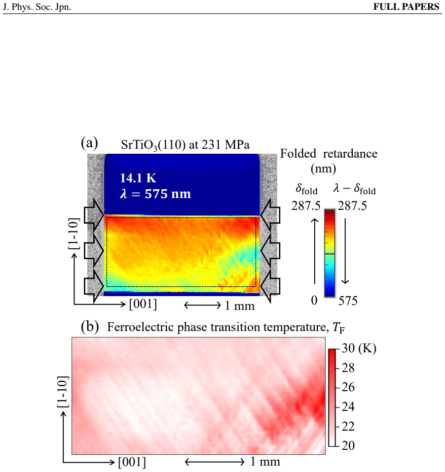
D. Andrienko, J. Mol. Liquids267, 520 (2018). 25/80 J. Phys. Soc. Jpn.FULL PAPERS 𝛿fold 287.5 575 SrTiO3(110) at 231 MPa [001] [1-10] 14.1 K 𝝀 = 𝟓𝟕𝟓 𝐧𝐦 1 mm 0 287.5 𝜆 − 𝛿fold Folded retardance (nm) 20 22 24 26 28 30 (K) (b) Ferroelectric phase transition temperature, 𝑇F (a) 1 mm[001] [1-10] Fig. 1.(Color online) (a) Folded optical retardance image (384×28...
2018
discussion (0)
Sign in with ORCID, Apple, or X to comment. Anyone can read and Pith papers without signing in.