Online Spectral Deflation for State Constrained Optimal Control Problems
Pith reviewed 2026-06-26 21:55 UTC · model grok-4.3
The pith
A single full-domain reference Schur complement supplies reusable low eigenmodes that accelerate CG solves of every parameter-dependent inactive-set system by 55 to 98 percent.
A machine-rendered reading of the paper's core claim, the machinery that carries it, and where it could break.
Core claim
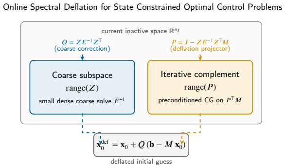
Low eigenmodes of one fixed full-domain reference Schur complement remain effective deflation vectors after they are restricted to each parameter-dependent inactive set. When these restricted modes are used inside an A-DEF2 deflation framework for Jacobi-preconditioned CG, iteration counts drop by 55 to 98 percent on diffusion, convection-diffusion, nonlinear thermal, and conjugate-heat-transfer benchmarks. The method therefore replaces repeated expensive rebuilds of preconditioners or factorizations with a single offline eigensolve whose output is reused for every active-set instance.
What carries the argument
The reusable A-DEF2 deflation basis obtained by restricting low eigenmodes of a single full-domain reference Schur complement to each new inactive set.
If this is right
- The same reference basis works without modification on diffusion, convection-diffusion, nonlinear thermal, and conjugate-heat-transfer problems.
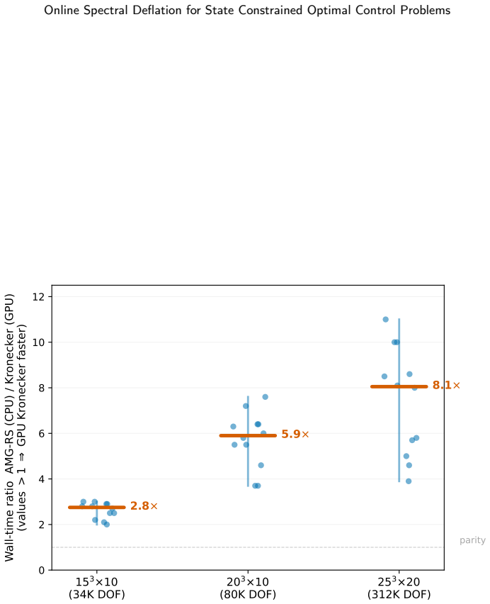
- GPU wall-time gains appear because the reference basis is built once while competing solver structures must be rebuilt per instance.
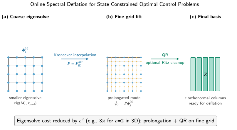
- Coarse-grid or analytical reference modes can amortize the offline cost inside a single parameter sweep.
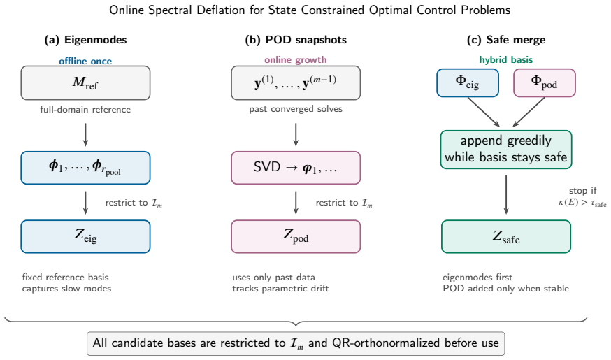
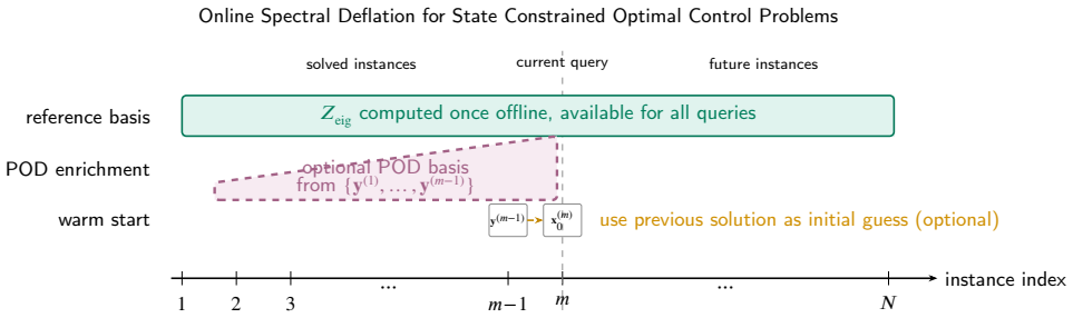
- The framework admits POD enrichment and Rayleigh-Ritz reselection while still preserving the exact inactive-set operator.
Where Pith is reading between the lines
- The spectral-coherence argument may apply to other active-set problems whose inactive sets evolve with a parameter, such as obstacle or contact problems.
- If the restricted reference modes remain accurate, similar deflation could be tested on time-dependent or stochastic control problems where the active set evolves continuously rather than parametrically.
- Pairing the deflation with a stronger base preconditioner than Jacobi could produce further gains, though the paper isolates the contribution of the deflation step itself.
Load-bearing premise
Low eigenmodes computed on the full-domain reference Schur complement remain effective deflation vectors after they are restricted to each parameter-dependent inactive set.
What would settle it
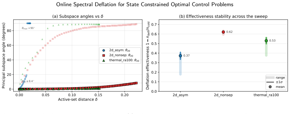
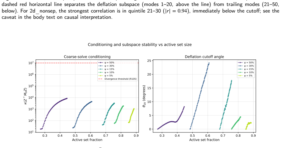
A benchmark instance in which the principal angles between the restricted reference modes and the true low eigenmodes of the new inactive-set operator become large enough that the deflation iteration count exceeds that of plain Jacobi-preconditioned CG.
Figures

read the original abstract
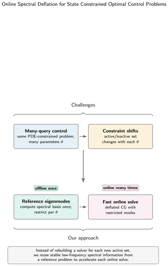
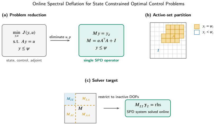
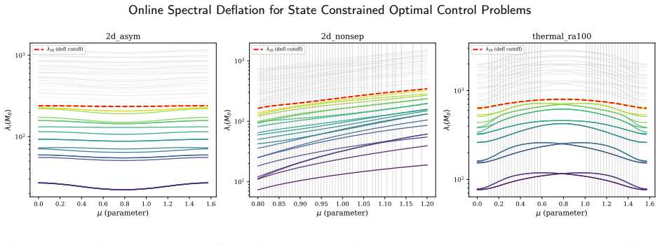
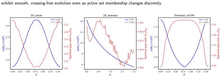
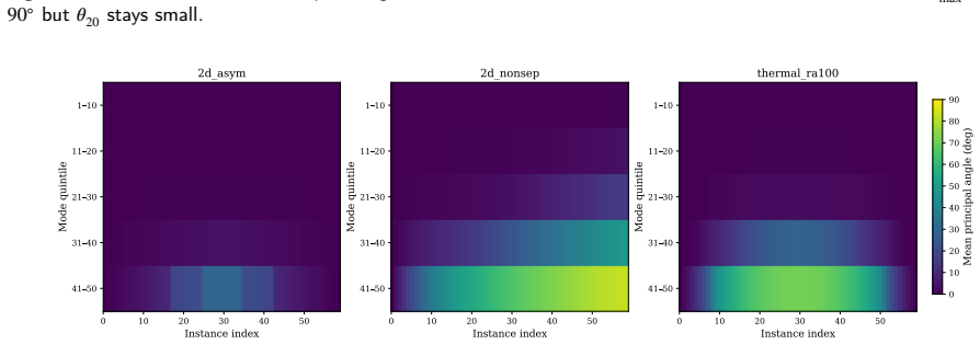
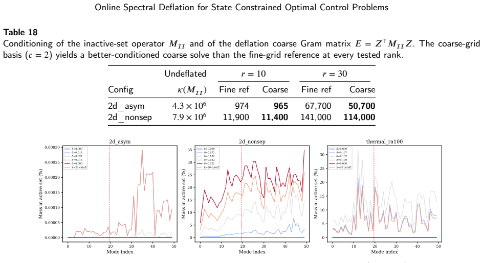
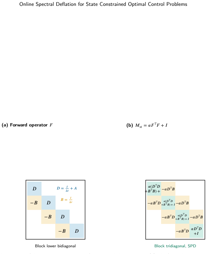
Parametric PDE-constrained optimal control with pointwise state constraints requires repeated solution of restricted Schur-complement systems on parameter-dependent inactive sets. In a primal active-set method, each inactive-set system is symmetric positive definite, but the active set can change nonsmoothly with the parameter. The resulting operator may vary in dimension, sparsity pattern, and spectrum, limiting reuse of sparse factorizations, multigrid hierarchies, and Krylov information. We propose a reusable spectral-deflation strategy anchored to one full-domain reference Schur complement. Low reference eigenmodes are computed once, restricted online to each inactive set, and used as an A-DEF2 deflation basis for Jacobi-preconditioned CG. The framework also supports POD enrichment, Rayleigh-Ritz reselection, coarse-grid or analytical reference modes, and conditioning safeguards. Given the active set, the method preserves the high-fidelity inactive-set system and solves it to the prescribed CG tolerance; it accelerates the linear algebra rather than replacing the optimal-control solve with a surrogate. We explain the method through a spectral-coherence view, motivated by interlacing and perturbation arguments and assessed with principal-angle diagnostics. Across diffusion, convection-diffusion, nonlinear thermal, and conjugate-heat-transfer benchmarks, deflation reduces CG iterations by about 55 to 98 percent. GPU deployments also show wall-time gains over CPU sparse-direct and algebraic-multigrid baselines, because the reference basis is built once whereas competing solver structures are rebuilt per instance. Coarse-grid or analytical modes amortize the offline cost within a single parameter sweep; fine-grid eigensolves remain more precompute-limited. Timings isolate the inactive-set linear-solve kernel; reducing the active-set outer loop is outside the present scope.
Editorial analysis
A structured set of objections, weighed in public.
Referee Report
Summary. The paper proposes a reusable spectral-deflation preconditioner for the sequence of symmetric positive definite Schur-complement systems that arise inside a primal active-set solver for parametric PDE-constrained optimal control problems with pointwise state constraints. Low eigenmodes are computed once on a single full-domain reference Schur complement, restricted online to each parameter-dependent inactive set, and employed as an A-DEF2 deflation basis inside Jacobi-preconditioned CG. The method is motivated by spectral-coherence, interlacing and perturbation arguments, assessed via principal-angle diagnostics, and reported to reduce CG iterations by 55–98 % on diffusion, convection-diffusion, nonlinear thermal and conjugate-heat-transfer benchmarks while preserving the original high-fidelity inactive-set operator and solving it to the prescribed tolerance.
Significance. If the restricted reference modes remain effective deflation vectors across the full range of inactive-set configurations encountered in a parameter sweep, the approach would amortize the dominant precomputation cost and yield substantial wall-time savings for repeated high-fidelity solves inside active-set optimal-control loops, particularly on GPU hardware. The framework’s support for POD enrichment, Rayleigh-Ritz reselection and analytical reference modes is a practical strength.
major comments (2)
- [spectral-coherence view / principal-angle diagnostics] The central iteration-reduction claim (55–98 %) rests on the assertion that low eigenmodes of the single full-domain reference Schur complement remain effective A-DEF2 vectors after restriction to each parameter-dependent inactive-set operator. The spectral-coherence section motivates this via interlacing and perturbation bounds, yet supplies no worst-case analysis or quantitative thresholds on principal angles when the inactive set is small, disconnected or topologically dissimilar from the reference; without such guarantees the reported savings cannot be asserted uniformly.
- [numerical results / benchmark descriptions] Although the abstract states that the method “preserves the high-fidelity inactive-set system and solves it to the prescribed CG tolerance,” the manuscript reports no quantitative verification (e.g., comparison of optimal-control objective values, constraint violation norms, or solution differences with and without deflation) that the deflation step does not degrade accuracy relative to a direct or AMG solve of the same inactive-set system.
minor comments (2)
- [GPU timings / baseline comparisons] Baseline solver details (exact AMG hierarchy construction, fill-in levels, and convergence tolerances) are not tabulated; this makes it difficult to reproduce the reported wall-time comparisons.
- [abstract and results tables] The phrase “about 55 to 98 percent” should be replaced by precise per-benchmark percentages together with the number of CG iterations and the corresponding reference values.
Simulated Author's Rebuttal
We thank the referee for the thoughtful comments on our manuscript. We address the major concerns below and outline the revisions we will make.
read point-by-point responses
-
Referee: [spectral-coherence view / principal-angle diagnostics] The central iteration-reduction claim (55–98 %) rests on the assertion that low eigenmodes of the single full-domain reference Schur complement remain effective A-DEF2 vectors after restriction to each parameter-dependent inactive-set operator. The spectral-coherence section motivates this via interlacing and perturbation bounds, yet supplies no worst-case analysis or quantitative thresholds on principal angles when the inactive set is small, disconnected or topologically dissimilar from the reference; without such guarantees the reported savings cannot be asserted uniformly.
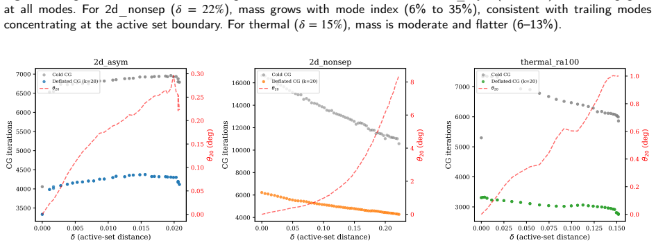
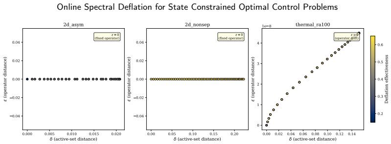
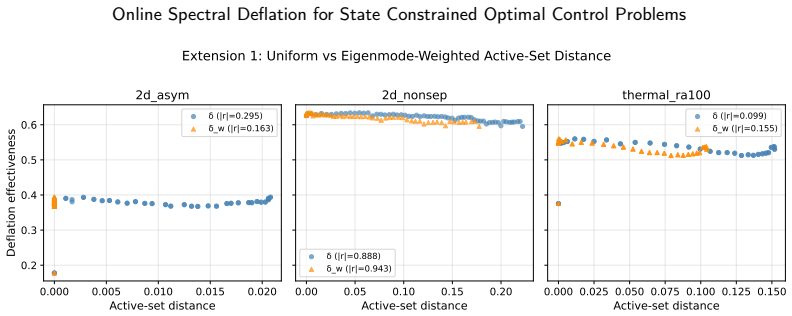
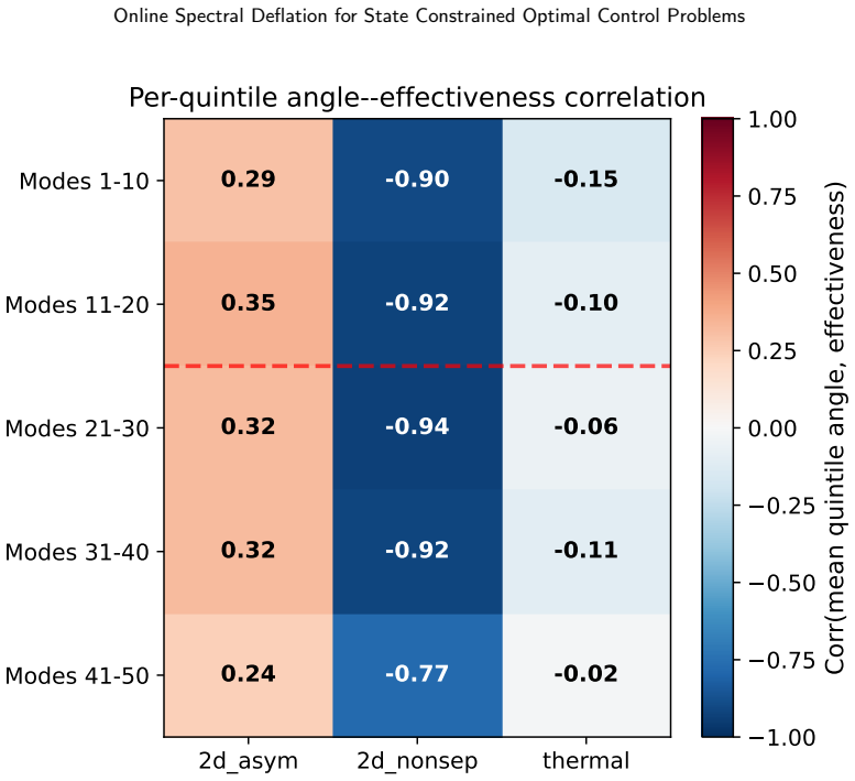
Authors: We agree that a rigorous worst-case analysis for arbitrary inactive-set configurations is not provided. Our spectral-coherence arguments based on interlacing and perturbation theory offer insight into why the reference modes remain effective, and the principal-angle diagnostics in the manuscript quantify the alignment for the benchmark problems. These benchmarks include varying inactive-set sizes and topologies arising from different parameter values. In the revised version we will expand the discussion to include additional principal-angle plots for the most dissimilar inactive sets encountered and clarify that the 55-98% iteration reductions are empirical observations for the tested problem families rather than a uniform guarantee. revision: partial
-
Referee: [numerical results / benchmark descriptions] Although the abstract states that the method “preserves the high-fidelity inactive-set system and solves it to the prescribed CG tolerance,” the manuscript reports no quantitative verification (e.g., comparison of optimal-control objective values, constraint violation norms, or solution differences with and without deflation) that the deflation step does not degrade accuracy relative to a direct or AMG solve of the same inactive-set system.
Authors: The deflation is used strictly as a preconditioner inside CG, which is converged to the same tolerance on the exact inactive-set matrix; therefore the computed solution satisfies the same residual criterion as a direct or AMG solve. Nevertheless, we acknowledge that explicit verification of the downstream optimal-control quantities would be valuable. We will add a new subsection or table in the numerical results section that compares the optimal objective values, maximum constraint violations, and L2 solution differences for selected parameter instances solved with and without deflation (using a direct solver as reference). revision: yes
Circularity Check
No circularity: reference eigenmodes and spectral arguments are independent of online instances
full rationale
The paper's core construction computes low eigenmodes once from a single full-domain reference Schur complement (independent of any parameter-dependent inactive set), then restricts them for A-DEF2 deflation. Justification rests on interlacing/perturbation arguments and principal-angle diagnostics rather than any fitted parameter, self-definition, or self-citation chain. No equation or claim reduces the reported iteration savings to a quantity defined by the method itself; the inactive-set system remains the exact high-fidelity operator. This is the common case of a self-contained algorithmic proposal whose central claims do not collapse by construction.
Axiom & Free-Parameter Ledger
axioms (2)
- standard math The inactive-set Schur complement remains symmetric positive definite for each active-set configuration.
- domain assumption Low eigenmodes of the full-domain reference operator provide useful deflation information after restriction to subsets.
Reference graph
Works this paper leans on
-
[1]
arXiv preprint arXiv:2606.13429
A scalable deflated conjugate gradient solver for the time-dependent pseudo-stress Stokes problem. arXiv preprint arXiv:2606.13429 . Candès, E.J., Romberg, J.K., Tao, T.,
-
[2]
Communications on Pure and Applied Mathematics 59, 1207–1223
Stable signal recovery from incomplete and inaccurate measurements. Communications on Pure and Applied Mathematics 59, 1207–1223. Casas,E.,1993. Boundarycontrolofsemilinearellipticequationswithpointwisestateconstraints. SIAMJournalonControlandOptimization31, 993–1006. Choi, Y., Boncoraglio, G., Anderson, S., Amsallem, D., Farhat, C., 2020a. Gradient-based...
1993
-
[3]
arXiv preprint arXiv:1909.11320
Accelerating design optimization using reduced order models. arXiv preprint arXiv:1909.11320 . Choi, Y.S.,
arXiv 1909
-
[4]
SIAM Journal on Matrix Analysis and Applications 34, 495–518
A framework for deflated and augmented Krylov subspace methods. SIAM Journal on Matrix Analysis and Applications 34, 495–518. doi:10.1137/110820713. Gong, W., Tan, Z.,
-
[5]
doi:10.1007/s10915-024-02747-3. Gutknecht, M.H.,
-
[6]
Applied Numerical Mathematics 41, 155–177
BoomerAMG: A parallel algebraic multigrid solver and preconditioner. Applied Numerical Mathematics 41, 155–177. doi:10.1016/S0168-9274(01)00115-5. Hestenes,M.R.,Stiefel,E.,1952. Methodsofconjugategradientsforsolvinglinearsystems. JournalofresearchoftheNationalBureauofStandards 49, 409–436. Hesthaven, J.S., Rozza, G., Stamm, B.,
-
[7]
The American mathematical monthly 111, 157–159
Cauchy’s interlace theorem for eigenvalues of hermitian matrices. The American mathematical monthly 111, 157–159. Ito,K.,Kunisch,K.,2003. Semi-smoothNewtonmethodsforstate-constrainedoptimalcontrolproblems. Systems&ControlLetters50,221–228. Kadeethum et al.:Preprint submitted to ElsevierPage 69 of 70 Online Spectral Deflation for State Constrained Optimal ...
2003
-
[8]
SIAM Journal on Scientific Computing 35, A1847–A1879
A trust-region algorithm with adaptive stochastic collocation for PDE optimization under uncertainty. SIAM Journal on Scientific Computing 35, A1847–A1879. Kunisch,K.,Volkwein,S.,2001. Galerkinproperorthogonaldecompositionmethodsforparabolicproblems. NumerischeMathematik90,117–148. Langer,U.,Steinbach,O.,Tröltzsch,F.,Yang,H.,2021. Space-timefiniteelementd...
2001
-
[9]
ARPACK Users’ Guide: Solution of Large-Scale Eigenvalue Problems with Implicitly Restarted Arnoldi Methods. SIAM, Philadelphia, PA. doi:10.1137/1.9780898719628. Leugering, G., Engell, S., Griewank, A., Hinze, M., Rannacher, R., Schulz, V., Ulbrich, M., Ulbrich, S. (Eds.),
-
[10]
arXiv preprint arXiv:2605.07828
NSPOD: Accelerating Krylov solvers via DeepONet-learned POD subspaces. arXiv preprint arXiv:2605.07828 . Li, Y., Zikatanov, L.T., Zuo, C.,
-
[11]
Fourier Neural Operator for Parametric Partial Differential Equations
Reduced Krylov basis methods for parametric partial differential equations. SIAM Journal on Numerical Analysis 63, 976–999. doi:10.1137/24M1661236. Li,Z.,Kovachki,N.B.,Azizzadenesheli,K.,Liu,B.,Bhattacharya,K.,Stuart,A.M.,Anandkumar,A.,2020. Fourierneuraloperatorforparametric partial differential equations. arXiv preprint arXiv:2010.08895 . Lu, L., Jin, P...
work page internal anchor Pith review Pith/arXiv arXiv doi:10.1137/24m1661236 2020
-
[12]
doi:10.1038/s42256-021-00302-5 Lu Lu, Raphaël Pestourie, Steven G
Learning nonlinear operators via DeepONet based on the universal approximation theorem of operators. Nature Machine Intelligence 3, 218–229. doi:10.1038/s42256-021-00302-5. McBane, S., Choi, Y.,
-
[13]
SIAM Journal on Numerical Analysis 24, 355–365
Deflation of conjugate gradients with applications to boundary value problems. SIAM Journal on Numerical Analysis 24, 355–365. Parks,M.L.,deSturler,E.,Mackey,G.,Johnson,D.D.,Maiti,S.,2006. RecyclingKrylovsubspacesforsequencesoflinearsystems. SIAMJournal on Scientific Computing 28, 1651–1674. Patankar, S.,
2006
-
[14]
Physics-informed neural networks: A deep learning framework for solving forward and inverse problems involving nonlinear partial differential equations. Journal of Computational Physics 378, 686–707. doi:10.1016/j.jcp.2018.10
-
[15]
OptimalsolversforPDE-constrainedoptimization
Rees,T.,Dollar,H.S.,Wathen,A.J.,2010. OptimalsolversforPDE-constrainedoptimization. SIAMJournalonScientificComputing32,271–298. Ruge, J.W., Stüben, K.,
2010
-
[16]
SIAM Journal on Scientific Computing 21, 1909–1926
A deflated version of the conjugate gradient algorithm. SIAM Journal on Scientific Computing 21, 1909–1926. Schöberl,J.,Zulehner,W.,2007. SymmetricindefinitepreconditionersforsaddlepointproblemswithapplicationstoPDE-constrainedoptimization problems. SIAM Journal on Matrix Analysis and Applications 29, 752–773. Soodhalter, K.M., Szyld, D.B., Xue, F.,
1909
-
[17]
arXiv preprint arXiv:2605.20639
Time-dependent pde-constrained optimization via weak-form latent dynamics. arXiv preprint arXiv:2605.20639 . Tröltzsch, F.,
-
[18]
International Journal for Numerical Methods in Engineering 69, 2441–2468
Large-scale topology optimization using preconditioned Krylov subspace methods with recycling. International Journal for Numerical Methods in Engineering 69, 2441–2468. Zahr,M.J.,Farhat,C.,2015. Progressiveconstructionofaparametricreduced-ordermodelforPDE-constrainedoptimization. InternationalJournal for Numerical Methods in Engineering 102, 1111–1135. Ka...
2015
discussion (0)
Sign in with ORCID, Apple, or X to comment. Anyone can read and Pith papers without signing in.